Chapter 1 Introductory Example

Statistics is the science of learning from data. But what is “Bayesian” statistics? This chapter provides a relatively simple and brief example of a Bayesian statistical analysis. As you work through the example, think about: What aspects are familiar? What features are new or different? Think big picture for now; we’ll fill in lots of details later.

Example 1.1 Suppose we’re interested in the proportion of all current Cal Poly students who have ever read at least one book in the Harry Potter series. We’ll refer to this proportion as the “population proportion”.

1. What are some challenges to computing the population proportion? How could we estimate it?

2. What are the possible values of the population proportion?

3. Which one of the following do you think is the most plausible value of the population proportion? Record your value in the plot on the board. \[ 0 \quad 0.1 \quad 0.2 \quad 0.3 \quad 0.4 \quad 0.5 \quad 0.6 \quad 0.7 \quad 0.8 \quad 0.9 \quad 1 \]

4. Sketch the plot of guesses here. What seems to be the consensus? What do we think are the most plausible values of the population proportion? Somewhat plausible? Not plausible?

5. The plot just shows our guesses for the population proportion. How could we estimate the actual population proportion based on data?

6. We will treat the roughly 30 students in our class as a random sample from the population of current Cal Poly students. But before collecting the data, let’s consider what might happen.

   Suppose that the actual population proportion is 0.5. That is, suppose that 50% of current Cal Poly students have read at least one Harry Potter book. How many students in a random sample of 30 students would you expect to have read at least one Harry Potter book? Would it necessarily be 15 students? How could you use a coin to simulate how many students in a random sample of 30 students might have read at least one Harry Potter book?

7. Now suppose the actual population proportion is 0.1. How would the previous part change?

8. Using your choice for the most plausible value of the population proportion, simulate how many students in a random sample of 30 students might have read at least one Harry Potter book. Repeat to get a few hypothetical samples, using your guess for the most plausible value of the population proportion, and record your results in the plot. (Here is one applet you can use.)

9. Why are there more dots corresponding to a proportion of 0.4 than to a proportion of 0.9?

10. How could we get an even clearer picture of what might happen?

11. Sketch the plot that we created. The plot illustrates two sources of uncertainty or variability. What are these two sources?

12. So far, everything we’ve considered is what might happen in a class of 30 students. Now let’s see what is actually true for our class. What proportion of students in the class have read at least one Harry Potter book? Is the proportion of all current Cal Poly students who have read at least one Harry Potter book necessarily equal to the sample proportion?

13. Remember that we started with guesses about which values of the population proportion were more plausible than others, and we used these guesses to get a picture of what might happen in samples. How can we reconsider the plausibility of the possible values of the population proportion in light of the sample data that we actually observed?

14. Given the observed sample proportion, what can we say about the plausible values of the population proportion? How has our assessment of plausibility changed from before observing the sample data?

15. What elements of the analysis are similar to the kinds of statistical analysis you have done before? What elements are new or different?

\iffalse{} Solution. to Example 1.1

Show/hide solution

1. It would be extremely challenging to survey all Cal Poly students. Even if we were able to obtain contact information for all students, many students would not respond to the survey. Instead, we can take a sample of Cal Poly students, collect data for students in the sample, and use the proportion of students in the sample who have read at least one Harry Potter book as a starting point to estimate the population proportion.

2. The population proportion could possibly be any value in the interval [0, 1]. Between 0% and 100% of current Cal Poly students have read at least one Harry Potter book.

3. There is no right answer for what you think is most plausible. Maybe you have a lot of friends that have read at least one Harry Potter book, so you might think the population proportion is 0.8. Maybe you don’t know anyone who has read at least one Harry Potter book, so you might think the population proportion is 0.1. Maybe you have no idea and you just guess that the population proportion is 0.5. Everyone has their own background information which influences their initial assessment of plausibility.

4. Results for the class will vary, but Figure 1.1 shows an example. The consensus for the class in Figure 1.1 is that values of 0.3, 0.4, and 0.5 are most plausible, 0.2 and 0.6 less so, and values close to 0 or 1 are not plausible.

5. We could use our class of 30 students as a sample, ask each student if they have read at least one Harry Potter book, and find the proportion of students in our class who have read at least one Harry Potter book.

6. If the actual population proportion is 0.5, we would expect around 15 students in a random sample of 30 students to have read at least one Harry Potter book. However, there would be natural sample-to-sample variability. To get a sense of this variability we could:

   • Flip a fair coin. Heads represents a student who has read at least one Harry Potter book; Tails, not.
   • A set of 30 flips represents one hypothetical random sample of 30 students.
   • The number of the 30 flips that land on Heads represents one hypothetical value of the number of students in a random sample of 30 students who have read at least one Harry Potter book.
   • Repeat the above process to get many hypothetical values of the number of students in a random sample of 30 students who have read at least one Harry Potter book, assuming that the population proportion is 0.5.

7. If the population proportion is 0.1 we would expect around 3 students in a random sample of 30 students to have read at least one Harry Potter book. Again, there would be natural sample-to-sample variability. To get a sense of this variability we could:

   • Roll a fair 10-sided die. A roll of 1 represents a student who has read at least one Harry Potter book; all other rolls, not.
   • A set of 30 rolls represents one hypothetical random sample of 30 students.
   • The number of the 30 rolls that land on 1 represents one hypothetical value of the number of students in a random sample of 30 students who have read at least one Harry Potter book.
   • Repeat the above process to get many hypothetical values of the number of students in a random sample of 30 students who have read at least one Harry Potter book, assuming that the population proportion is 0.1.

8. Figure 1.2 shows the number of students who have read at least one Harry Potter book in 5 hypothetical samples assuming the population proportion is 0.5, and in 5 hypothetical samples assuming the population proportion is 0.1.

9. Results for the class will vary. In the scenario in Figure 1.1, a value of 0.4 was initially more plausible than a value of 0.9. There were more students who thought 0.4 was the most plausible value than 0.9. So the value 0.4 gets more “weight” in the simulation than 0.9. The plot on the left in Figure 1.3 reflects the results of a simulation where every student who plotted a dot in Figure 1.1 simulates 5 random samples of size 30, using their guess for the population proportion.

10. Repeat the simulation process to get many hypothetical samples for each value for the population proportion, reflecting differences in initial plausibility. Imagine each student simulated 10000 samples instead of 5. The plot on the right in Figure 1.3 displays the results.

11. The plot illustrates natural sample-to-sample variability in the sample proportion for a given value of the population proportion. The plot also illustrates the uncertainty in the value of the population proportion. That is, the population proportion has a distribution of values determined by our relative initial plausibilities.

12. Results will vary. We’ll assume that 9 out of 30 students have read at least one Harry Potter book, for a sample proportion of \(9/30 = 0.3\). While we hope that 0.3 is close to the proportion of all current Cal Poly students who have read at least one Harry Potter book, because of natural sample-to-sample variability the sample proportion is not necessarily equal to the population proportion.

13. The simulation demonstrated what might happen in a sample of size 30. Now we can zoom in on what actually did happen. Among the samples in the simulation that resulted in 9 students having read a Harry Potter book, what were the corresponding population proportions?

14. Figure 1.4 displays the results based on the smaller scale simulation in the plot on the left in Figure 1.3, in which every initial guess for the sample proportion generated five hypothetical samples of size 30. Now we focus on samples that resulted in a sample proportion of 9/30, the observed sample proportion. The middle plot displays the population proportions correspoding to samples with a sample proportion of 9/30. The distribution of all the dots in the middle plot illustrates our initial plausibility. The plot on the right displays only the green dots, which correspond to samples with a sample proportion of 9/30. The distribution in the plot on the right reflects a reassessment of the plausibilities of possible values of the population proportion given the observed sample proportion of 9/30 and the simulation results. Among the simulated samples that resulted in a sample proportion of 9/30, the population proportion was much more likely to be 0.3 than to be 0.5.

    Figure 1.5 displays the same analsyis based on the full simulation from the plot on the right in Figure 1.3. The plot on the right in Figure 1.5 compares the initial plausibilities to the plausibilities revised upon observing a sample proportion of 9/30. Initially, the values 0.3, 0.4, and 0.5 were roughly equally plausible, and more plausible than any other value. After observing a sample proportion of 9/30:

    • 0.3 is the most plausible value of the population proportion
    • 0.3 is about two times more plausible than the next most plausible value, 0.4
    • 0.3 and 0.4 together account for the bulk of plausibility.
    • Initially, 0.5 was much more plausible than 0.2, but given the observed data 0.2 is now more plausible than 0.5 (though neither is very plausible)

15. Familiar elements include:

    • using sample statistics to make inference about population parameters
    • reflecting sample-to-sample variability of statistics, for a given value of the population parameter
    • using simulation to analyze data and understand ideas

    New elements include:

    • Quantifying the uncertainty of the population proportion with relative plausibilities of possible values
    • Treating the population proportion as a variable with a distribution determined by the relative plausibilities
    • Conditioning on the observed data and revising our assessment of plausibilities

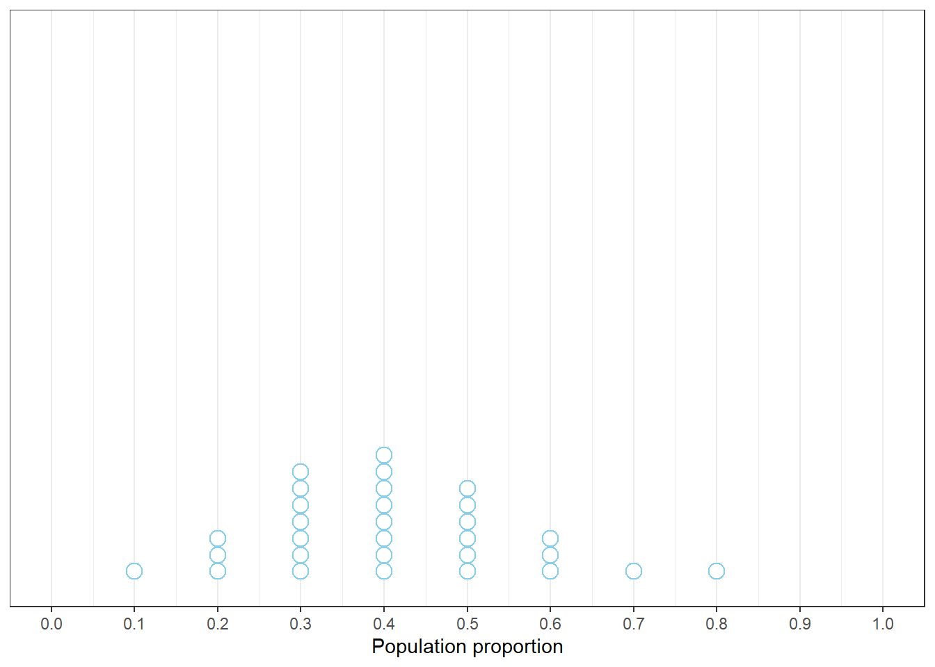
Figure 1.1: Example plot of the guesses of 30 students for the most plausible value of the proportion of current Cal Poly students who have read at least one Harry Potter book.

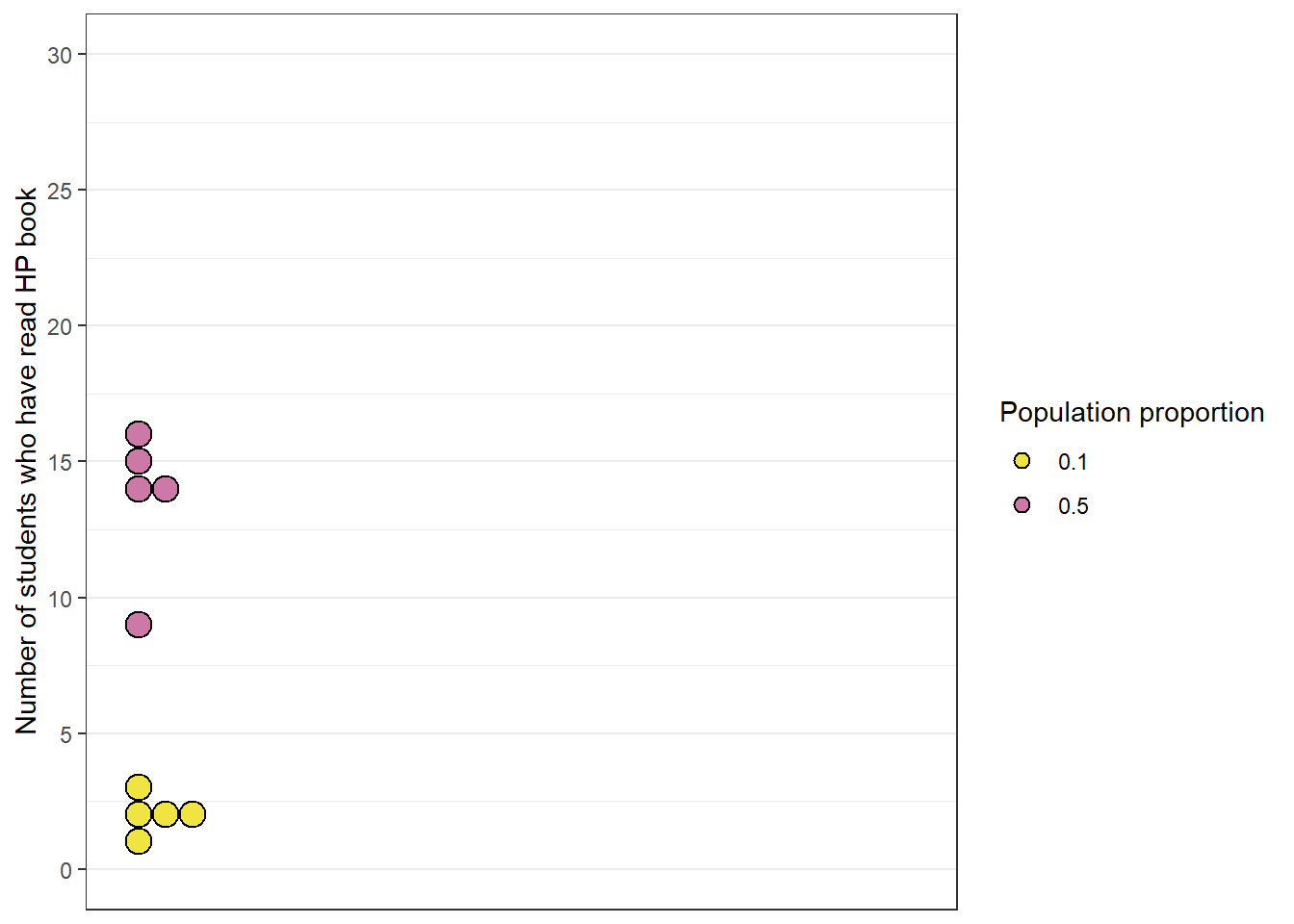
Figure 1.2: Number of students who have read at least one Harry Potter book in hypothetical samples of size 30. Five samples simulated assuming the population proportion is 0.1 (yellow), and five samples simulated assuming the population proportion is 0.5 (purple).

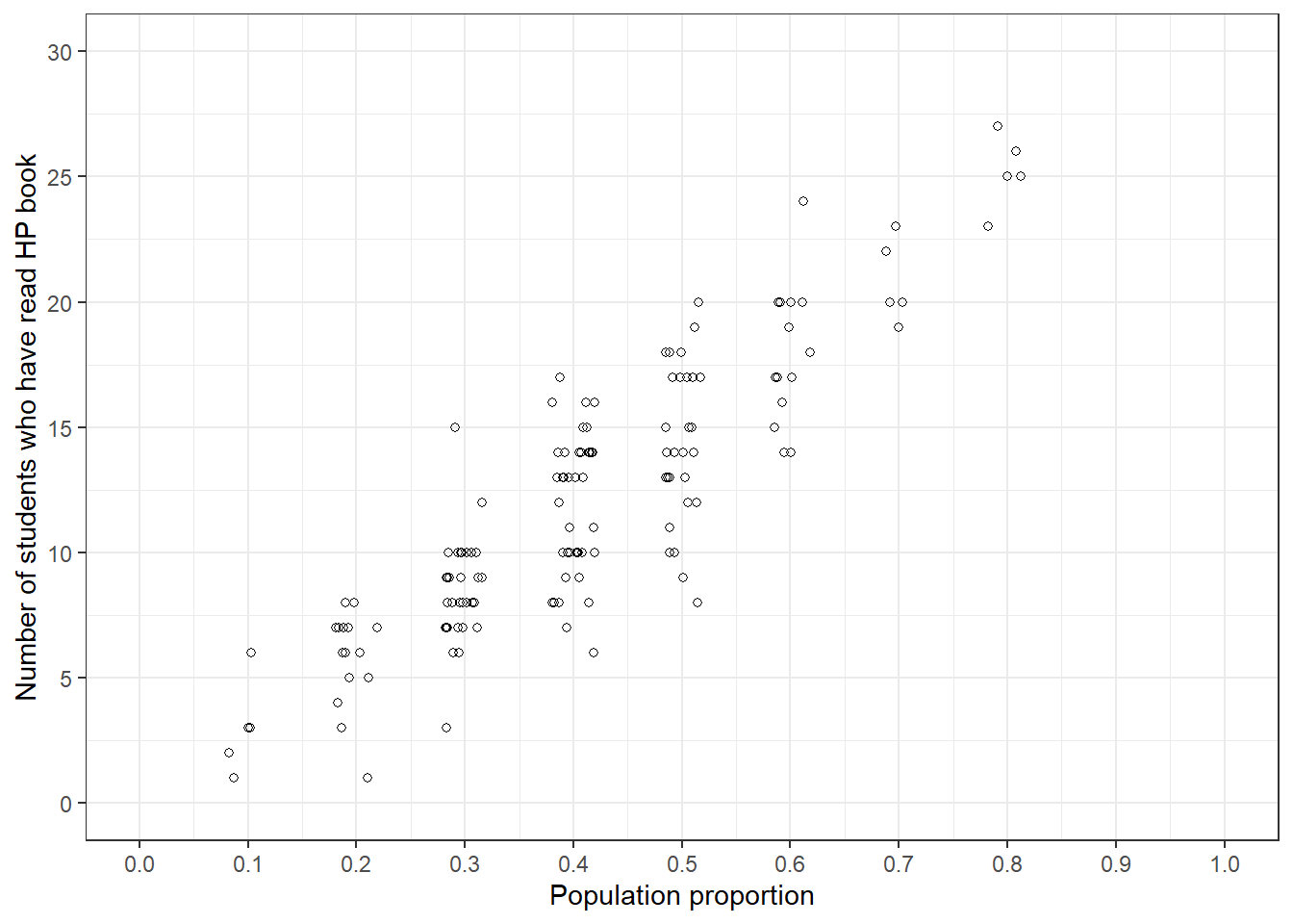
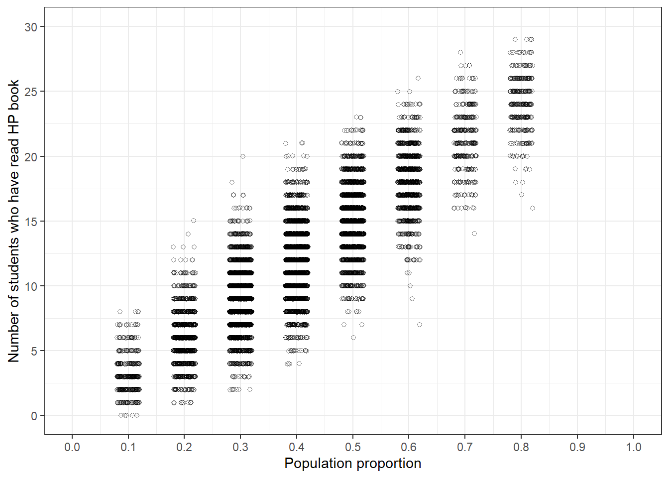
Figure 1.3: Simulation of the number of students who have read at least one Harry Potter book in hypothetical samples of size 30, reflecting initial plausibility of values of the population proportion from Figure 1.1. Left: 5 hypothetical samples for each guess for the population proportion. Right: 10000 hypothetical samples for each guess for the population proportion.

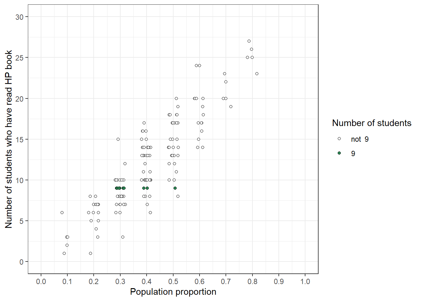
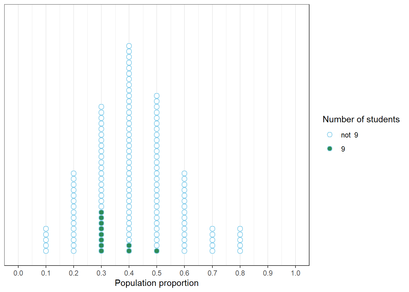
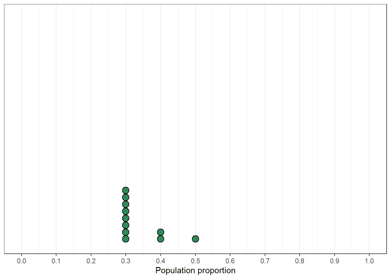
Figure 1.4: Left: Simulation results from the plot on the left in Figure 1.3 highlighting samples with a sample proportion of 9/30. Middle: Comparison of initial distribution of population proportion with conditional distribution of population proportion given a sample proportion of 9/30. Right: Distribution reflecting relative plausibility of possible values of the population proportion after observing a sample of 30 students in which 9 have read at least one Harry Potter book.

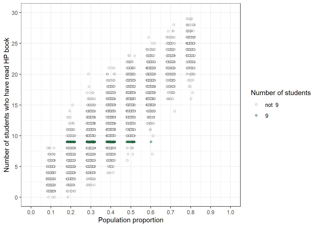
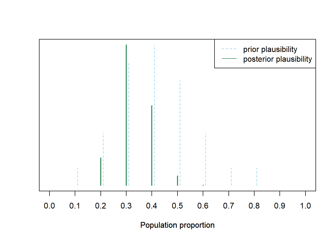
Figure 1.5: Left: Simulation results from the plot on the right in Figure 1.3 highlighting samples with a sample proportion of 9/30. Right: Distribution reflecting relative plausibility of possible values of the population proportion, both “prior” plausibility (blue) and “posterior” plausibility after observing a sample of 30 students in which 9 have read at least one Harry Potter book (green).