7.2 Prior predictive tuning

Prior distributions of parameters quantify uncertainty about parameters before observing data. Considering prior predictive distributions of possible samples under the proposed model can help tune prior distributions of parameters.

Example 7.5 Suppose we want to estimate \(\theta\), the population mean hours of sleep on a typical night for Cal Poly students. Assume that sleep hours for individual students follow a Normal distribution with unknown mean \(\theta\) and known standard deviation 1.5 hours. (Known population SD is an unrealistic assumption that we use for simplicity here.)

Suppose we want to use a fairly uninformative prior for \(\theta\), so we choose a Uniform distribution on the interval [4, 12].

Simulate sleep hours for 10000 Cal Poly students under this model and make a histogram of the simulated values.
According to this model, (approximately) what percent of students sleep less than 5 hours a night? More than 11? Do these values seem reasonable?

\iffalse{} Solution. to Example 7.5

First simulate a value \(\theta\) from the Uniform(4, 12) distribution. Then given \(\theta\) simulate a value \(y\) from a Normal(\(\theta\), 1.5) distribution. Repeat many times to get many \((\theta, y)\) pairs and summarize the \(y\) values.
```
N_sim = 10000

theta = runif(N_sim, 4, 12)

sigma = 1.5
y = rnorm(N_sim, theta, sigma)

hist(y, xlab = "Sleep hours")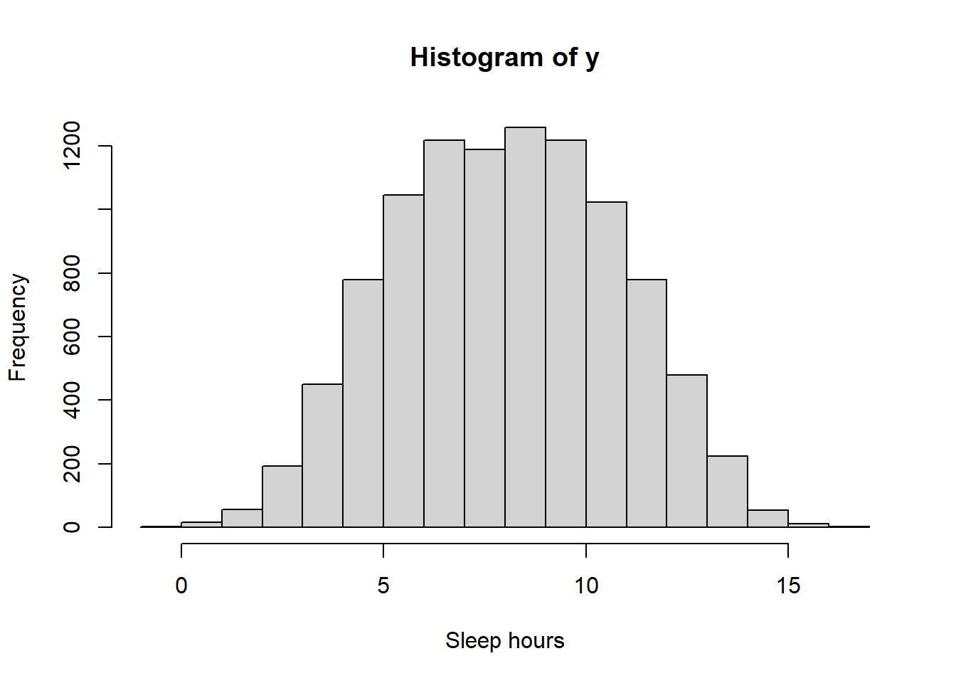
```
```
sum(y < 5) / N_sim
```
```
## [1] 0.1499
```
```
sum(y > 11) / N_sim
```
```
## [1] 0.1552
```
According to this model, about 15 percent of students sleep fewer than 5 hours on a typical night, and about 16 percent of students sleep more than 11 hours on a typical night. These values seem to be overestimates, indicating that perhaps the model isn’t the greatest.
It could be that the prior distribution is too uninformative. But it could also be that the assumptions of the data model are inadequate; perhaps a Normal distribution isn’t appropriate for sleep times. (Of course, the value \(\sigma\) could be also wrong, but here we’re assuming it’s known.)

In the previous example, it was helpful to think about the distribution of sleep hours for individual students when formulating prior beliefs about the population mean. In general, it is often easier to think in terms of the scale of the data (individual sleep hours) rather than the scale of the parameters (mean sleep hours).

Prior predictive distributions “live” on the scale of the data, and are sometimes easier to interpret than prior distributions themselves. It is often helpful to tune prior distributions indirectly via prior predictive distributions rather than directly. We can choose a prior distribution for parameters, simulate a prior predictive distribution for the data given this prior, and consider if the distribution of possible data values seems reasonable given our background knowledge about the variable and context. If not, we can choose another prior and repeat the process until we have suitably “tuned” the prior.

Remember, the prior does not have to be perfect; there is no perfect prior. However, if a particular prior gives rise to obviously unreasonable data values (e.g., negative sleep hours) we should try to improve it. It’s always a good idea to consider prior predictive distributions when formulating a prior distribution for parameters.