Chapter 2 Ideas of Bayesian Reasoning
In this section we’ll look a closer look at the example from the previous section. In particular, we’ll inspect the simulation process and results in more detail. We’ll also consider a more “realistic” scenario.
In the previous section, each student identified a “most plausible” value. We collected these guesses to form a “wisdom of crowds” measure of initial plausibility.
However, your own initial assessment of the plausibility of the different values could involve much more than just identifying the most plausible value. What was your next most plausible value? How much less plausible was it? What about the other values and their relative plausibilities?
In the example below we’ll start with an assessment of plausibility. We’ll discuss later how you might obtain such an assessment. For now, focus on the big picture: we start with some initial assessment of plausibility before observing data, and we want to update that assessment upon observing some data.
Example 2.1 Suppose we’re interested in the proportion of all current Cal Poly students who have ever read at least one book in the Harry Potter series. We’ll refer to this proportion as the “population proportion” and denote it as \(\theta\) (the Greek letter “theta”).
We’ll start by considering only the values 0.1, 0.2, 0.3, 0.4, 0.5, 0.6 as initially plausible for the population proportion \(\theta\). Suppose that before collecting sample data, our prior assessment is that:
- 0.2 is four times more plausible than 0.1
- 0.3 is two times more plausible than 0.2
- 0.3 and 0.4 are equally plausible
- 0.2 and 0.5 are equally plausible
- 0.1 and 0.6 are equally plausible
Construct a table to represent this prior distribution and sketch a plot of it.
Discuss what the prior distribution from the previous part represents.
If we simulate many values of the population proportion according to the above distribution, on what proportion of repetitions would we expect to see a value of 0.1? If we conduct 260000 repetitions of the simulation, on how many repetitions would we expect to see a value of 0.1? Repeat for the other plausible values to make a table of what we would expect the simulation results to look like. (For now, we’re ignoring simulation variability; just consider expected values.)
The “prior” describes our initial assessment of plausibility of possible values of the population proportion prior to observing data. Now suppose we observe a sample of 30 students in which 9 students have read at least one HP book. We want to update our assessment of the population proportion in light of the observed data.
Suppose that the actual population proportion is \(\theta=0.1\). How could we use simulation to determine the likelihood of observing 9 students who have read at least one HP book in a sample of 30 students? How could we use math? (Hint: what is the probability distribution of the number of “successes” in a sample of size 30 when \(\theta=0.1\)?)
Recall the simulation with 260000 repetitions that we started above. Consider the 10000 repetitions in which the population proportion is 0.1. Suppose that for each of these repetitions we simulate the number of students in a class of 30 who have read at least one HP book. On what proportion of these repetitions would we expect to see a sample count of 9? On how many of these 10000 repetitions would we expect to see a sample count of 9?
Repeat the previous part for each of the possible values of \(\theta\): \(0.1, \ldots, 0.6\). Add two columns to the table: one column for the likelihood of observing a count of 9 in a sample of size 30 for each value of \(\theta\), and one column for the expected number of repetitions in the simulation which would result in the count of 9.
Consider just the repetitions that resulted in a simulated sample count of 9. What proportion of these repetitions correspond to a population proportion of 0.1? Of 0.2? Continue for the other possible values of \(\theta\) to construct this posterior distribution, and sketch a plot of it.
After observing a sample of 30 Cal Poly students with a proportion of 9/30=0.3 who have read at least one Harry Potter book, what can we say about the plausibility of possible values of the population proportion? How has our assessment of plausibility changed from before observing the sample data?
Prior to observing data, how many times more plausible is a value of 0.3 than 0.2 for the population proportion \(\theta\)?
Recall that we observed a sample count of 9 in a sample of size 30. How many times more likely is a count of 9 in a sample of size 30 when the population proportion \(\theta\) is 0.3 than when it is 0.2?
After observing data, how many times more plausible is 0.3 than 0.2 for the population proportion \(\theta\)?
How are the values from the three previous parts related?
The relative plausibilities allow us to draw the shape of the plot below: the spike for 0.2 is four times as high as the one for 0.1; the spike for 0.3 is two times higher than the spike for 0.2, etc. To make a distribution we need to rescale the heights, maintaining the relative ratios, so that they add up to 1. It helps to consider one value as a “baseline”; we’ll choose 0.1 (but it doesn’t matter which value is the baseline). Assign 1 “unit” of plausibility to the value 0.1 Then 0.6 also gets 1 unit of plausibility. The values 0.2 and 0.5 each receive 4 units of plausibility, and the values 0.3 and 0.4 each receive 8 units of plausibility. The six values account for 26 total units of plausibility. Divide the units by 26 to obtain values that sum to 1. See the “Prior” column in the table below. Check that the relative ratios are maintained; for example, the rescaled prior plausibility of 0.308 for 0.3 is two times larger than the rescaled prior plausibility of 0.154 for 0.2.
Population proportion Prior “Units” Prior 0.1 1 0.0385 0.2 4 0.1538 0.3 8 0.3077 0.4 8 0.3077 0.5 4 0.1538 0.6 1 0.0385 Total 26 1.0000 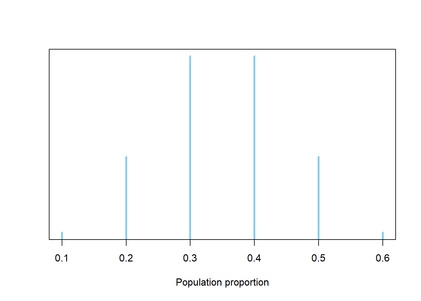
The parameter \(\theta\) is an uncertain quantity. We are considering this quantity as a random variable, and using distributions to describe our degree of uncertainty. The prior distribution represents our degree of uncertainty, or our assessment of relative plausibility of possible values of the parameter, prior to observing data.
The relative prior plausibility of 0.1 is 1/26, so we would expect to see a value of 0.1 for \(\theta\) on about 3.8% of repetitions. If we conduct 260000 repetitions of the simulation, we would expect to see a value of 0.1 for \(\theta\) on about 10000 repetitions.
Population proportion Prior “Units” Prior Number of reps 0.1 1 0.0385 10000 0.2 4 0.1538 40000 0.3 8 0.3077 80000 0.4 8 0.3077 80000 0.5 4 0.1538 40000 0.6 1 0.0385 10000 Total 26 1.0000 260000 If the population proportion is 0.1 we would expect around 3 students in a random sample of 30 students to have read at least one Harry Potter book. Again, there would be natural sample-to-sample variability. To get a sense of this variability we could:
- Roll a fair 10-sided die. A roll of 1 represents a student who has read at least one Harry Potter book; all other rolls, not.
- A set of 30 rolls represents one hypothetical random sample of 30 students.
- The number of the 30 rolls that land on 1 represents one hypothetical value of the number of students in a random sample of 30 students who have read at least one Harry Potter book.
- Repeat the above process to get many hypothetical values of the number of students in a random sample of 30 students who have read at least one Harry Potter book, assuming that the population proportion is 0.1.
If \(Y\) is the number of students in the same who have read at least one HP book, then \(Y\) has a Binomial(30, \(\theta\)) distribution. If \(\theta=0.1\) then \(Y\) has a Binomial(30, 0.1) distribution. If \(\theta=0.1\) the probability that \(Y=9\) is \(\binom{30}{9}(0.1^9)(0.9^{21})=0.0016\), which can be computed using
dbinom(9, 30, 0.1)in R.dbinom(9, 30, 0.1)## [1] 0.001565From the previous part, the likelihood of observing a count of 9 in a sample of size 30 when \(\theta=0.1\) is 0.0016. If \(\theta=0.1\) then we would expect to observe a sample count of 9 in about 0.16% of samples. In the 10000 repetitions with \(\theta=0.1\), we would expect to observe a count of 9 in about \(10000 \times 0.0016 = 16\) repetitions.
See the table below. For example, if \(\theta=0.2\) then the likelihood of a sample count of 9 in a sample of size 30 is \(\binom{30}{9}(0.2^9)(0.8^{21})=0.068\), which can be computed using
dbinom(9, 30, 0.2). If \(\theta=0.2\) then we would expect to observe a sample count of 9 in about 6.8% of samples. In the 40000 repetitions with \(\theta=0.2\), we would expect to observe a count of 9 in about \(40000 \times 0.068 = 2703\) repetitions.In the table below, “Likelihood of 9” represents the probability of a sample count of 9 in a sample of size 30 computed for each possible value of \(\theta\). Note that this column does not sum to 1, as the values in this column do not comprise a probability distribution. Rather, the values in the likelihood column represent the probability of the same event (sample count of 9) computed under various different scenarios (different possible values of \(\theta\)).
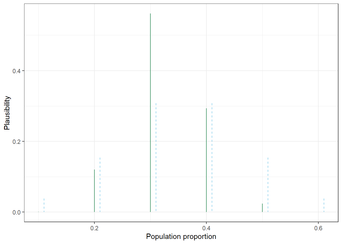
The “Repetitions with a count of 9” column corresponds to the green dots in Figure 1.5. The prior plausibilities and total number of repetitions are different between the two examples, but the process is the same. (The overall “Number of reps” column corresponds to all the dots.)
Population proportion Prior “Units” Prior Number of reps Likelihood of count of 9 Reps with count of 9 0.1 1 0.0385 10000 0.0016 16 0.2 4 0.1538 40000 0.0676 2703 0.3 8 0.3077 80000 0.1573 12583 0.4 8 0.3077 80000 0.0823 6582 0.5 4 0.1538 40000 0.0133 533 0.6 1 0.0385 10000 0.0006 6 Total 26 1.0000 260000 0.3227 22423 There were 22423 repetitions that resulted in a simulated sample count of 9. Of these, 16 correspond to a population proportion of 0.1. Therefore, the proportion of repetitions that resulted in a count of 9 that correspond to a proportion of 0.1 is 16 / 22423 = 0.0007. The proportion of repetitions that resulted in a count of 9 that correspond to a proportion of 0.2 is 2703 / 22423 = 0.1205. See the “Posterior” column in the table below.
Population proportion Prior “Units” Prior Number of reps Likelihood of count of 9 Reps with count of 9 Posterior 0.1 1 0.0385 10000 0.0016 16 0.0007 0.2 4 0.1538 40000 0.0676 2703 0.1205 0.3 8 0.3077 80000 0.1573 12583 0.5612 0.4 8 0.3077 80000 0.0823 6582 0.2935 0.5 4 0.1538 40000 0.0133 533 0.0238 0.6 1 0.0385 10000 0.0006 6 0.0003 Total 26 1.0000 260000 0.3227 22423 1.0000 The plot below compares our prior plausibility (blue) and our posterior plausibility (green) after observing the data. The values 0.3 and 0.4 initially were equally plausible for \(\theta\), but after observing a sample proportion of 0.3 the value 0.3 is now almost 2 times more plauible than a value of 0.4. The values 0.2, 0.3, 0.4 together accounted for about 77% of our initial plausibility, but after observing the data these three values now account for over 97% of our plausibility.
Our prior assessment was that a value of 0.3 is 2 times more plausible than 0.2 for the population proportion \(\theta\).
A count of 9 in a sample of size 30 is 0.1573 / 0.0676 = 2.33 times mores likely when the population proportion \(\theta\) is 0.3 than when it is 0.2.
After observing a count of 9 in a sample of size 30, a value of 0.3 is 0.5612 / 0.1205 = 4.66 times more plausible than 0.2 for the population proportion \(\theta\).
The ratio of the posterior plausibilities (4.66) is the product of the ratio of the prior plausibilities and the ratio of the likelihoods (2.33). In short, posterior is proportional to product of prior and likelihood.
What is the problem with considering only the values 0.1, 0.2, …, 0.6 as plausible? How could we resolve this issue?
Suppose we have a prior distribution that assigns initial relative plausibility to a fine grid of possible values of the population proportion \(\theta\), e.g., 0, 0.0001, 0.0002, 0.0003, …, 0.9999, 1. We then observe a sample count of 9 in a sample of size 30. Explain the process we would use to construct a table like the one in the previous example to find the posterior distribution of the population proportion \(\theta\).
How could we use the posterior distribution to fill in the blank in the following: “There is a [blank] percent chance that fewer than 50 percent of current Cal Poly students have read at least one HP book.”
What are some other questions of interest regarding \(\theta\)? How could you use the posterior distribution to answer them?
These six values are not the only possible values of \(\theta\). The parameter \(\theta\) is a proportion, which could take any value in [0, 1]. We really want a prior that assigns relative plausibility to all values in the continuous interval [0, 1]. One way to bridge the gap is to consider a fine grid of values in [0, 1], rather than all possible values.
We’ll consider the possible values of \(\theta\) to be \(0, 0.0001, 0.0002, 0.0003, \ldots, 0.9998, 0.9999, 1\) and assign a relative plausibility to each of these values. We’ll start with our assessment from the previous example: 0.1 and 0.6 are equally plausible, 0.2 is four times more plausible than 0.1, etc. We’ll assign plausibility to in between values by “smoothly connecting the dots”. In the plot below this is achieved with a Normal distribution, but the details are not important for now. Just understand that (1) we have expanded our grid of possible values of \(\theta\), and (2) we have assigned a relative plausibility to each of the possible values.
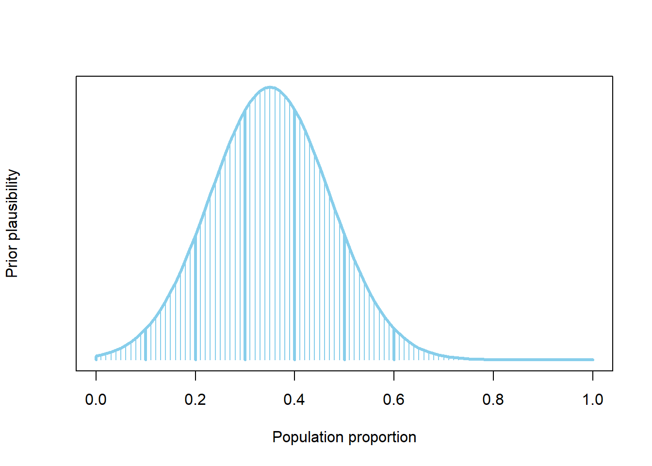
The table has one row for each possible value of \(\theta\): \(0, 0.0001, 0.0002, \ldots, 0.9999, 1\).
- Prior: There would be a column for prior plausibility, say corresponding to the plot above.
- Likelihood: For each value of \(\theta\), we would compute the likelihood of observing a sample count of 9 in a sample of size 30: \(\binom{30}{9}(\theta^9)(1-\theta)^{21}\) or
dbinom(9, 30, theta). - Product: For each value of \(\theta\), compute the product of prior and likelihood. This is essentially what we did in the previous example in the “Reps with a count of 9” column. Here we’re just not multiplying by the total number of repetitions.
- Posterior: The product column gives us the relative ratios. For example, the product column tells us that the posterior plausibility of 0.3 is 4.66 times greater than the posterior plausibility of 0.2. We simply need to rescale these values — by dividing by the sum of the product column — to obtain posterior plausibilities in the proper ratios that add up to one.
The following is some code; think of this as creating a spreadsheet. (Note that only a few select rows of the spreadsheet are displayed below.) We will explore code like this in much more detail as we go. For now, just notice that we can accomplish what we wanted in just a few lines of code.
# Possible values of theta
theta = seq(0, 1, 0.0001)


# Prior distribution
# Smoothly connect the dots using a Normal distribution
# Then rescale to sum to 1

prior = dnorm(theta, 0.35, 0.12) # prior "units" - relative values
prior = prior / sum(prior) # recale to sum to 1


# Likelihood
# Likelihood of observing sample count of 9 out of 30
# for each theta

likelihood = dbinom(9, 30, theta)


# Posterior
# Product gives relative posterior plausibilities
# Then rescale to sum to 1

product = prior * likelihood
posterior = product / sum(product)

# Put the columns together
bayes_table = data.frame(theta,
                     prior,
                     likelihood,
                     product,
                     posterior)

# Display a portion of the table
bayes_table %>%
  slice(seq(2001, 4001, 250)) %>% # selects a few rows to display
  kable(digits = 8)
theta prior likelihood product posterior 0.200 0.0001525 0.06756 0.00001030 0.0001204 0.225 0.0001936 0.10012 0.00001938 0.0002265 0.250 0.0002353 0.12981 0.00003055 0.0003570 0.275 0.0002740 0.15019 0.00004115 0.0004808 0.300 0.0003054 0.15729 0.00004803 0.0005613 0.325 0.0003259 0.15062 0.00004909 0.0005736 0.350 0.0003330 0.13285 0.00004424 0.0005170 0.375 0.0003259 0.10847 0.00003535 0.0004131 0.400 0.0003054 0.08228 0.00002512 0.0002936 The plot below displays the prior, likelihood1, and posterior. Notice that the likehood of the observed data is highest for \(\theta\) near 0.3, so our plausibility has “moved” in the direction of \(\theta\) near 0.3 after observing the data.
# The code below plots three curves
# One for each of prior, likelihood, posterior
# There are easier/better ways to do this

ggplot(bayes_table, aes(x = theta)) +
  geom_line(aes(y = posterior), col = "seagreen") +
  geom_line(aes(y = prior), col = "skyblue") +
  geom_line(aes(y = likelihood / sum(likelihood)), col = "orange") +
  labs(x = "Population proportion (theta)",
   y = "Plausibility",
   title = "Prior (blue), (Scaled) Likelihood (orange), Posterior (green)") +
  theme_bw()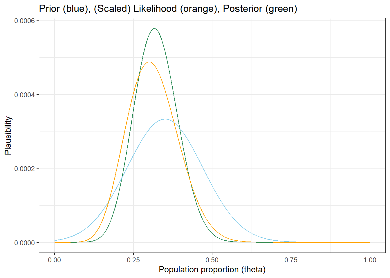
Sum the posterior plausibilities for \(\theta\) values between 0.5. We can see from the plot that almost all our plausibility is placed on values of \(\theta\) less than 0.5.
sum(posterior[theta < 0.5])## [1] 0.9939The posterior distribution gives us lots of information. We might be interested in questions like: “There is a [blank1] percent chance that between [blank2] and [blank3] percent of Cal Poly students have read a HP book.” For example, for 80 percent in blank1, we might compute the 10th percentile for blank2 and the 90th percentile for blank3. Using the spreadsheet, start from \(\theta=0\) and go down the table summing the posterior probabilities until they reach 0.1; the corresponding \(\theta\) value is the 10th percentile.
theta[max(which(cumsum(posterior) < 0.1))]## [1] 0.235We can find the 90th percentile similarly.
theta[max(which(cumsum(posterior) < 0.9))]## [1] 0.411There is an 80% chance that between 24% and 41% of Cal Poly students have read a HP book.