Chapter 17 Introduction to Markov Chain Monte Carlo (MCMC) Simulation

Bayesian data analysis is based on the posterior distribution of relevant parameters given the data. However, in many situations the posterior distribution cannot be determined analytically or via grid approximation. Therefore we use simulation to approximate the posterior distribution and its characteristics. But in many situations it is difficult or impossible to simulate directly from a distribution, so we turn to indirect methods.

Markov chain Monte Carlo (MCMC)³² methods provide powerful and widely applicable algorithms for simulating from probability distributions, including complex and high-dimensional distributions.

Example 17.1 A politician campaigns on a long east-west chain of islands³³. At the end of each day she decides to stay on her current island, move to the island to the east, or move to the island to the west. Her goal is to visit all the islands proportional to their population, so that she spends the most days on the most populated island, and proportionally fewer days on less populated islands. But, (1) she doesn’t know how many islands there are, and (2) she doesn’t know the population of each island. However, when she visits an island she can determine its population. And she can send a scout to the east/west adjacent islands to determine their population before visiting. How can the politician achieve her goal in the long run?

Suppose that every day, the politician makes her travel plans according to the following algorithm.

She flips a fair coin to propose travel to the island to the east (heads) or west (tails). (If there is no island to the east/west, treat it as an island with population zero below.)
If the proposed island has a population greater than that of the current island, then she travels to the proposed island.
If the proposed island has a population less than that of the current island, then:
- She computes \(a\), the ratio of the population of the proposed island to the current island.
- She travels to the proposed island with probability \(a\),
- And with probability \(1-a\) she spends another day on the current island.

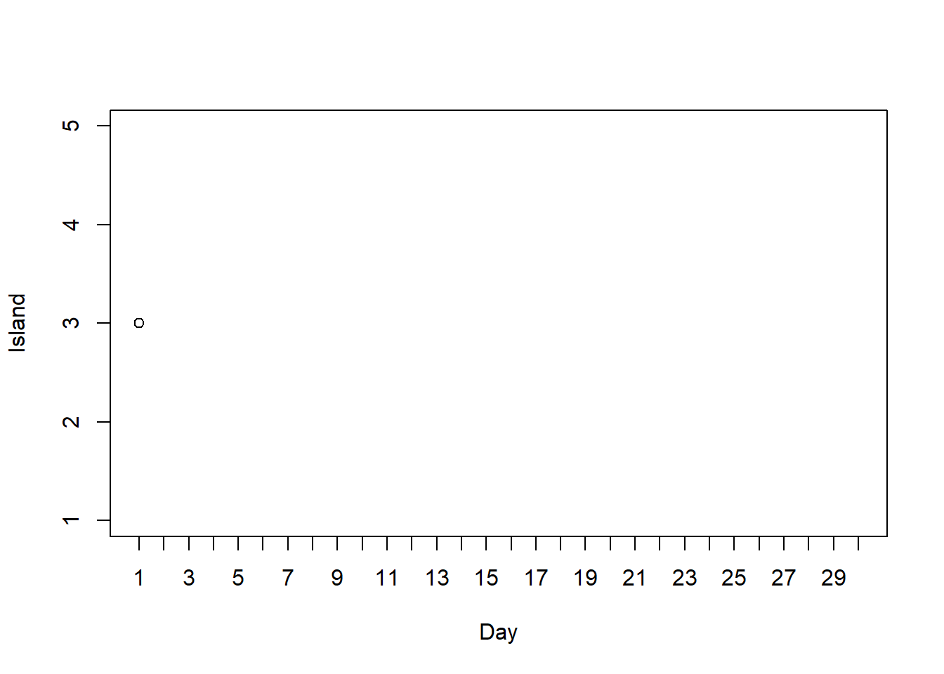
Suppose there are 5 islands, labeled \(1, \ldots, 5\) from west to east, and that island \(\theta\) has population \(\theta\) (thousand), and that she starts at island 3 on day 1. How could you use a coin and a spinner to simulate by hand the politician’s movements over a number of days? Conduct the simulation and plot the path of her movements.
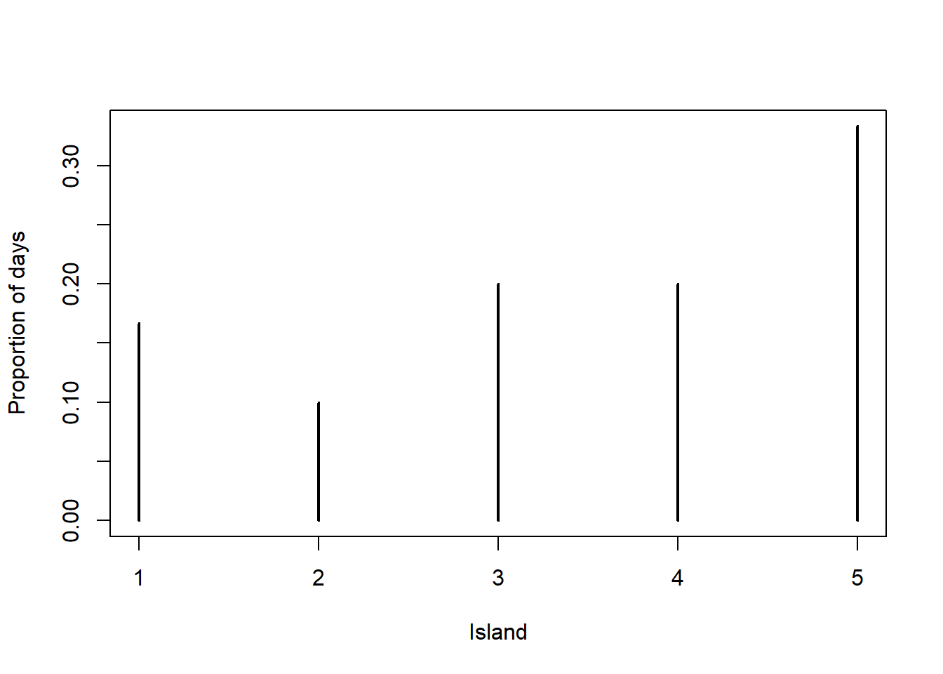
Construct by hand a plot displaying the simulated relative frequencies of days in each of the 5 islands.
Now write code to simulate the politician’s movements for many days. Plot the island path.
Plot the simulated relative frequencies of days in each of the 5 islands.
Recall the politician’s goal of visiting each island in proportion to its population. Given her goal, what should the plot from the previous part look like? Does the algorithm result in a reasonable approximation?
Suppose again that the number of islands and their populations is unknown, but that the population for island \(\theta\) is proportional to \(\theta^2 e^{-0.5\theta}\), where the islands are labeled from west to east 1, 2, \(\ldots\). Based on this information, can she implement her algorithm? That is, is it sufficient to know that the populations are in proportion to \(\theta^2 e^{-0.5\theta}\) without knowing the actual populations? In particular, is there enough information to compute the “acceptance probability” \(a\)?
Write code to run the algorithm for the previous situation and compare the simulated relative frequencies to the target distribution. Does the algorithm result in a reasonable approximation?
Why doesn’t the politician just always travel to or stay on the island with the larger population?
Is the next island visited dependent on the current island?
Is the next island visited dependent on how she got to the current island? That is, given the current island is her next island independent of her past history of previous movements?
What would happen if there were an island among the east-west chain with population 0? (For example, suppose there are 10 islands, she starts on island 1, and island 5 has population 0.) How could she modify her algorithm to address this issue?

\iffalse{} Solution. to Example 17.1

Starting at island \(\theta\), flip a coin to propose a move to either \(\theta-1\) or \(\theta+1\). If the proposed move is to \(\theta+1\), it will be accepted because the population is larger. If the proposed move is to \(\theta-1\) it will be accepted with probability \((\theta-1)/\theta\); otherwise the move will be rejected and she will stay in the current island.

For example, starting in island 3 she proposes a move to either island 2 or island 4. If the proposed move is to island 4, it is accepted and she moves to island 4. If the proposed move is to island 2, it is accepted with probability 2/3. If it is accepted she moves to island 2; otherwise she stays at island 3 for another day.

If she is on island 1 and she proposes a move to the west, the proposal is rejected (because the population of island “0” is 0) and she spends another day on island 1. Likewise if she proposes a move to the east from island 5.

The acceptance probabilities are \[\begin{align*} a(1\to 0) & = 0 & a(1\to 2) & =1\\ a(2\to 1) & = 1/2 & a(2\to 3) & =1\\ a(3\to 2) & = 2/3 & a(3\to 4) & =1\\ a(4\to 3) & = 3/4 & a(4\to 5) & =1\\ a(5\to 4) & = 4/5 & a(5\to 6) & =0\\ \end{align*}\]

Here is an example plot for 30 days.
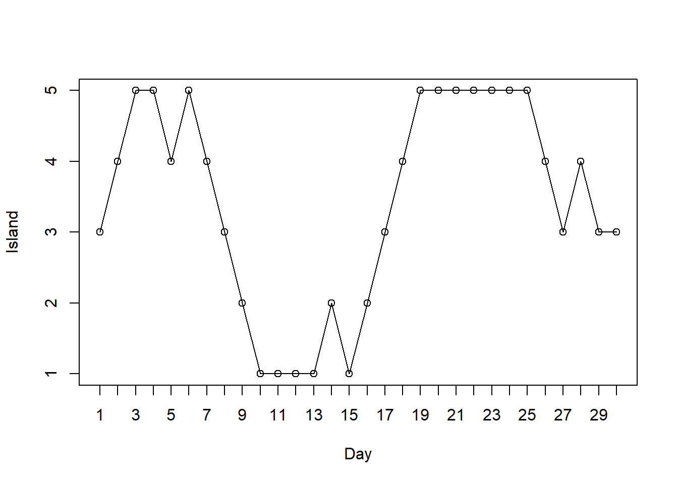
The plot below corresponds to the path from the previous plot.

Some code is below. There are different ways to implement this algorithm, but note the proposal and acceptance steps below.

n_states = 5
theta = 1:n_states
pi_theta = theta

n_steps = 10000
theta_sim = rep(NA, n_steps)
theta_sim[1] = 3 # initialize

for (i in 2:n_steps){
  current = theta_sim[i - 1]
  proposed = sample(c(current + 1, current - 1), size = 1, prob = c(0.5, 0.5))
  if (!(proposed %in% theta)){ # to correct for proposing moves outside of boundaries
proposed = current
  }
  a = min(1, pi_theta[proposed] / pi_theta[current])
  theta_sim[i] = sample(c(proposed, current), size = 1, prob = c(a, 1-a))
}

# trace plot
plot(1:n_steps, theta_sim, type = "l", ylim = range(theta), xlab = "Day", ylab = "Island")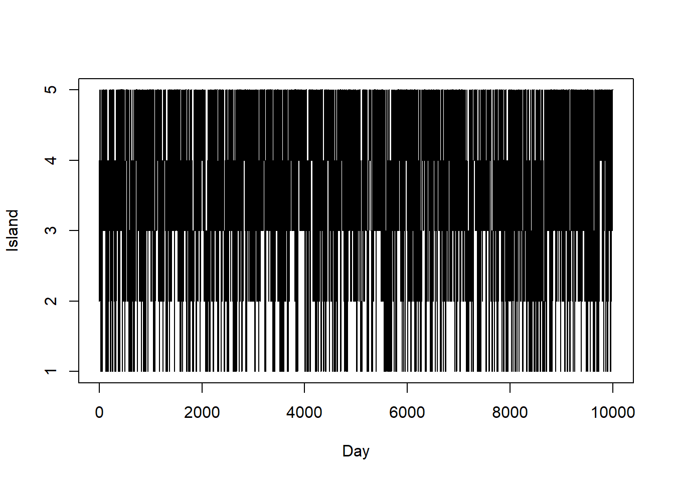

The plot below corresponds to the path from the previous plot.

plot(table(theta_sim) / n_steps, xlab = "Island", ylab = "Proportion of days")

points(theta, theta / 15, type = "o", col = "seagreen")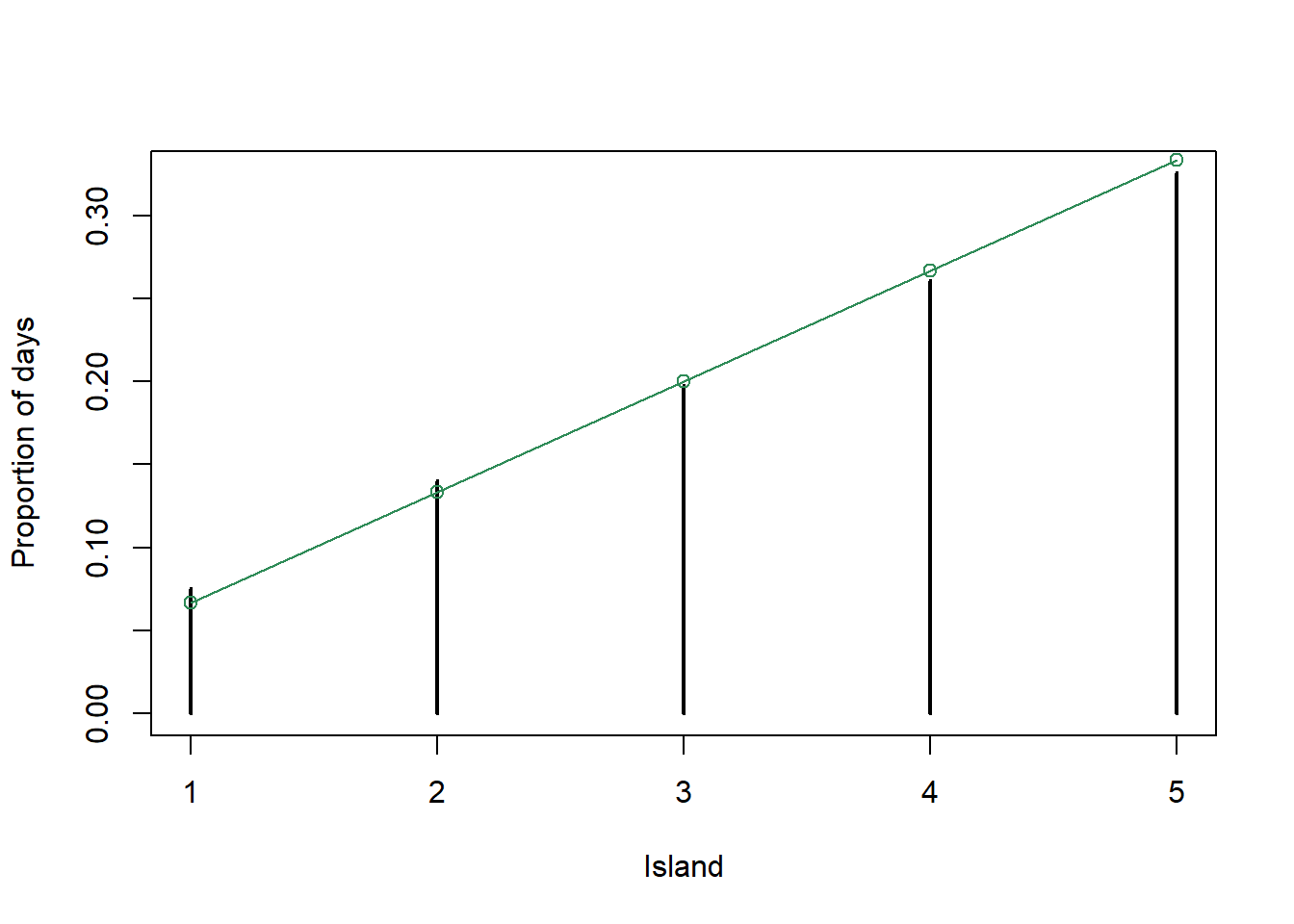

Since the population of island \(\theta\) is proportional to \(\theta\), the target probability distribution satisfies \(\pi(\theta)\propto \theta, \theta = 1, \ldots, 5\). That is, \(\pi(\theta) = \theta/15, \theta = 1, \ldots, 5\). This distribution is depicted in green in the previous plot. We see that the algorithm does produce a reasonable approximation.
She can still make east-west proposals with a coin flip. And she can still decide whether to accept the proportion based on relative population. If she is currently on island \(\theta_{\text{current}}\) and she proposes a move to island \(\theta_{\text{proposed}}\), she will accept the proposal with probability \[ a(\theta_{\text{current}}\to \theta_{\text{proposed}}) = \frac{\theta_{\text{proposed}}^2 e^{-0.5\theta_{\text{proposed}}}}{\theta_{\text{current}}^2 e^{-0.5_{\text{current}}}} \] In terms of running the algorithm it is sufficient to know that the populations are in proportion to \(\theta^2 e^{-0.5\theta}\) without knowing the actual populations.

See below; it seems like a reasonable approximation.

n_states = 30
theta = 1:n_states
pi_theta = theta ^ 2 * exp(-0.5 * theta) # notice: not probabilities


n_steps = 10000
theta_sim = rep(NA, n_steps)
theta_sim[1] = 1 # initialize

for (i in 2:n_steps){
  current = theta_sim[i - 1]
  proposed = sample(c(current + 1, current - 1), size = 1, prob = c(0.5, 0.5))
  if (!(proposed %in% theta)){ # to correct for proposing moves outside of boundaries
proposed = current
  }
  a = min(1, pi_theta[proposed] / pi_theta[current])
  theta_sim[i] = sample(c(proposed, current), size = 1, prob = c(a, 1-a))
}

# trace plot
plot(1:n_steps, theta_sim, type = "l", ylim = range(theta_sim), xlab = "Day", ylab = "Island")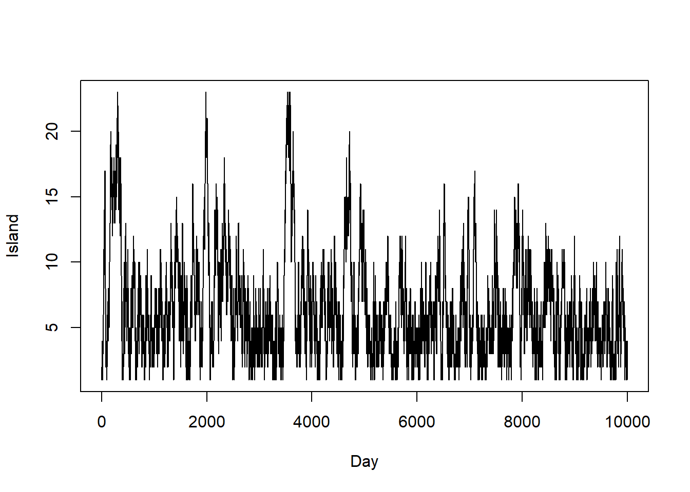

plot(table(theta_sim) / n_steps, xlab = "Island", ylab = "Proportion of days")

points(theta, pi_theta / sum(pi_theta), type = "o", col = "seagreen")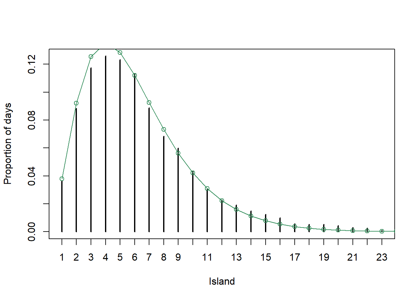

She wants to visit the islands in proportion to their population. So she still wants to visit the smaller islands, just not as often as the larger ones. But if she always move towards islands with larger populations, she would not visit the smaller ones at all.
Yes, the next island visited dependent on the current island. For example, if she is on island 3 today, tomorrow she can only be on island 2, 3, or 4.
No the next island visited is not dependent on how she got to the current island. The proposals and acceptance probability only depend on the current state, and not past states (given the current state).
With only east-west proposals, since she would never visit an island with population 0 (because the acceptance probability would be 0), she could never get to islands on the other side. She could modify her algorithm to cast a wider net in her proposals, instead of just proposing moves to adjacent islands.

The goal of a Markov chain Monte Carlo method is to simulate from a probability distribution of interest. In Bayesian contexts, the distribution of interest will usually be the posterior distribution of parameters given data.

A Markov chain is a random process that exhibits a special “one-step” dependence structure. Namely, conditional on the most recent value, any future value is conditionally independent of any past values. In a Markov chain: “Given the present, the future is conditionally independent of the past.” Roughly, in terms of simulating the next value of a Markov chain, all that matters is where you are now, not how you got there.

The idea of MCMC is to build a Markov chain whose long run distribution — that is, the distribution of state visits after a large number of “steps” — is the probability distribution of interest. Then we can indirectly simulate a representative sample from the probability distribution of interest, and use the simulated values to approximate the distribution and its characteristics, by running an appropriate Markov chain for a sufficiently large number of steps. The Markov chain does not need to be fully specified in advance, and is often constructed “as you go” via an algorithm like a “modified random walk”. Each step of the Markov chain typically involves

A proposal for the next state, which is generated according to some known probability distribution or mechanism,
A decision of whether or to accept the proposal. The decision usually involves probability
- With probability \(a\), accept the proposal and step to the next state
- With probability \(1-a\), reject the proposal and remain in the current state for the next step.

In principle, proposals can be fairly naive and not related to the target distribution (though in practice choice of proposal is very important since it affects computational efficiency). Furthermore, the target distribution of interest only needs to be specified up to a constant of proportionality, and the state space of possible values does not need to be fully specified in advance.

The island hopping example illustrated an MCMC algorithm for a discrete parameter \(\theta\). Recall that most parameters in statistical models take values on a continuous scale, so most posterior distributions are continuous distributions. MCMC simulation can also be used to approximate the posterior distribution and related characteristics for continuous distributions.

The following examples illustrates how MCMC can be used to approximate the posterior distribution in a Beta-Binomial setting. Of course, this scenario can be handled analytically and so MCMC is not necessary. However, it will help to see how the ideas work in a familiar context where an analytical solution is available.

Example 17.2 Suppose we wish to estimate \(\theta\), the proportion of Cal Poly students who have read a non-school related book in 2022. Assume a Beta(1, 3) prior distribution for \(\theta\). In a sample of 25 Cal Poly students, 4 have read a book in 2021. We’ll use MCMC to approximate the posterior distribution of \(\theta\).

Without actually computing the posterior distribution, what can we say about it based on the assumptions of the model?
What are the possible “states” that we want our Markov chain to visit?
Given a current state \(\theta_\text{current}\) how could we propose a new value \(\theta_{\text{proposed}}\), using a continuous analog of “random walk to neighboring states”?
How would we decide whether to accept the proposed move? How would we compute the probability of accepting the proposed move?
Suppose the current state is \(\theta_\text{current}=0.20\) and the proposed state is \(\theta_\text{proposed}=0.15\). Compute the probability of accepting this proposal.
Suppose the current state is \(\theta_\text{current}=0.20\) and the proposed state is \(\theta_\text{proposed}=0.25\). Compute the probability of accepting this proposal.
Write code to run the algorithm and plot the simulated values of \(\theta\).
What is the posterior distribution? Does the distribution of simulated values of \(\theta\) provide a reasonable approximation to the posterior distribution?

\iffalse{} Solution. to Example 17.2

Since posterior is proportional to likelihood times prior, we know that \[\begin{align*} \pi(\theta|y = 4) & \propto f(y=4|\theta)\pi(\theta)\\ & \propto \left(\theta^4(1-\theta)^{25-4}\right)\left(\theta^{1-1}(1-\theta)^{3-1}\right) \end{align*}\]
\(\theta\) takes values in (0, 1) so each possible value in (0, 1) is a state.
There are different approaches, but here’s a common one. We want to propose a new state in the neighborhood of the current state. Given \(\theta_{\text{current}}\), propose \(\theta_{\text{proposed}}\) from a \(N(\theta_{\text{current}}, \delta)\) distribution where the standard deviation \(\delta\) represents the size of the “neighborhood”. For example, if \(\theta_{\text{current}} = 0.5\) and \(\delta=0.05\) then we would draw the proposal from the \(N(0.5, 0.05)\) distribution, so there’s a 68% chance the proposal is between 0.45 and 0.55 and a 95% chance that it’s between 0.40 and 0.60.
Remember, the goal is to approximate the posterior distribution, so we want to visit the \(\theta\) states in proportion to their posterior density. If the proposed state has higher posterior density than the current state, \(\pi(\theta_{\text{proposed}}|y=4) > \pi(\theta_{\text{current}}|y=4)\), then we accept the proposal. Otherwise, accept the proposal with a probability based on the relative posterior densities of the proposed and current states. That is, we accept the proposed move with probability \[ \scriptstyle{ a(\theta_\text{current}\to \theta_{\text{proposed}}) = \min\left(1,\, \frac{\pi(\theta_{\text{proposed}}|y=4)}{\pi(\theta_{\text{current}}|y=4)}\right) = \min\left(1,\, \frac{\left(\theta_{\text{proposed}}^4(1-\theta_{\text{proposed}})^{25-4}\right)\left(\theta_{\text{proposed}}^{1-1}(1-\theta_{\text{proposed}})^{3-1}\right)}{\left(\theta_{\text{current}}^4(1-\theta_{\text{current}})^{25-4}\right)\left(\theta_{\text{current}}^{1-1}(1-\theta_{\text{current}})^{3-1}\right)}\right) } \]
The posterior density is larger for the proposed state, so the proposed move is accepted with probability 1. \[ \scriptstyle{ a(0.20 \to 0.15) = \min\left(1,\, \frac{\pi(0.15|y=4)}{\pi(0.20|y=4)}\right) = \min\left(1,\, \frac{\left(0.15^4(1-0.15)^{25-4}\right)\left(0.15^{1-1}(1-0.15)^{3-1}\right)}{\left(0.20^4(1-0.20)^{25-4}\right)\left(0.20^{1-1}(1-0.20)^{3-1}\right)}\right) =1 } \]
```
(dbeta(0.15, 1, 3) * dbinom(4, 25, 0.15)) / (dbeta(0.2, 1, 3) * dbinom(4, 25, 0.2))
```
```
## [1] 1.276
```
The posterior density is smaller for the proposed state, so based on the ratio of the posterior densities, the proposed move is accepted with probability 0.553. \[ \scriptstyle{ a(0.20 \to 0.25) = \min\left(1,\, \frac{\pi(0.25|y=4)}{\pi(0.20|y=4)}\right) = \min\left(1,\, \frac{\left(0.25^4(1-0.25)^{25-4}\right)\left(0.25^{1-1}(1-0.25)^{3-1}\right)}{\left(0.20^4(1-0.20)^{25-4}\right)\left(0.20^{1-1}(1-0.20)^{3-1}\right)}\right) =0.553 } \]
```
(dbeta(0.25, 1, 3) * dbinom(4, 25, 0.25)) / (dbeta(0.2, 1, 3) * dbinom(4, 25, 0.2))
```
```
## [1] 0.5533
```

See below. The Normal distribution proposal can propose values outside of (0, 1), so we set \(\pi(\theta|y=4)\) equal to 0 for \(\theta\notin(0,1)\). This way, proposals to states outside (0, 1) will never be accepted.

n_steps = 10000
delta = 0.05

theta = rep(NA, n_steps)
theta[1] = 0.5 # initialize

# Posterior is proportional to prior * likelihood
pi_theta <- function(theta) {
  if (theta > 0 & theta < 1) dbeta(theta, 1, 3) * dbinom(4, 25, theta) else 0
}

for (n in 2:n_steps){
  current = theta[n - 1]
  proposed = current + rnorm(1, mean = 0, sd = delta)
  accept = min(1, pi_theta(proposed) / pi_theta(current))
  theta[n] = sample(c(current, proposed), 1, prob = c(1 - accept, accept)) 
}

# simulated values of theta
hist(theta, breaks = 50, freq = FALSE,
 xlab = "theta", ylab = "pi(theta|y = 4)", main = "Posterior Distribution")

# plot of theoretical posterior density of theta
x_plot= seq(0, 1, 0.0001)
lines(x_plot, dbeta(x_plot, 1 + 4, 3 + 25 - 4), col = "seagreen", lwd = 2)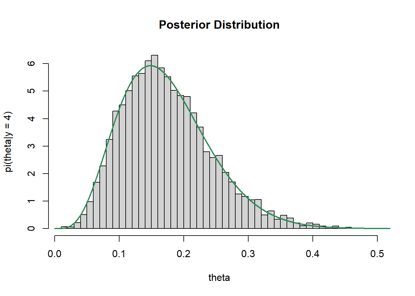

plot(1:100, theta[1:100], type = "o", xlab = "n", 
 ylab = expression(theta[n]), main = "First 100 steps")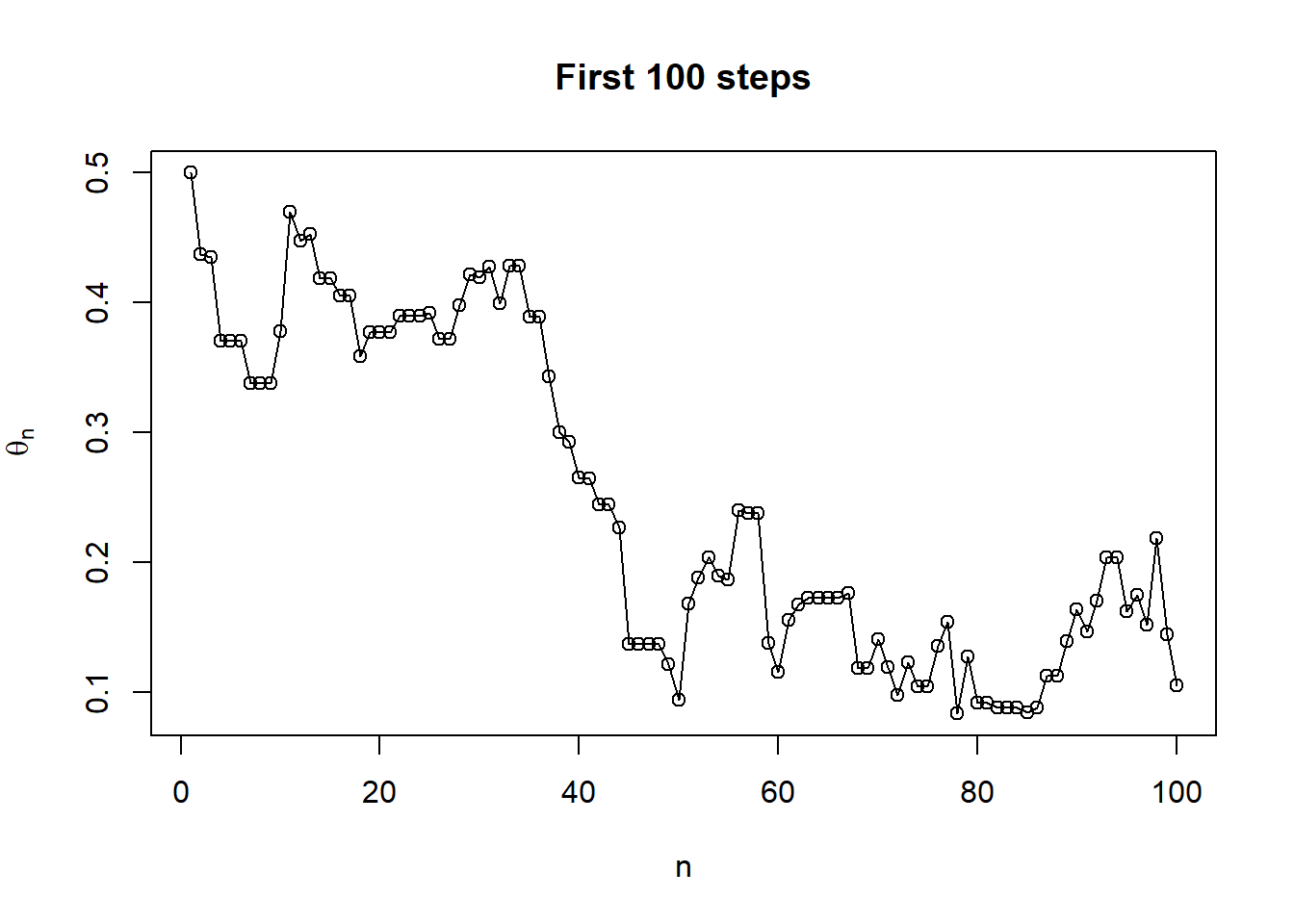

plot(1:n_steps, theta, type = "l", xlab = "n", 
 ylab = expression(theta[n]), main = "All steps")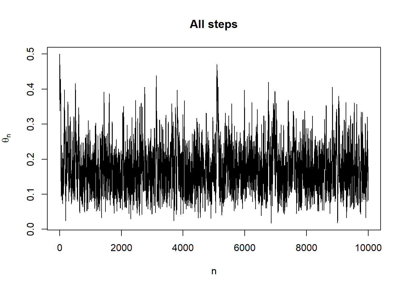

The theoretical posterior distribution is the Beta(5, 24) distribution, depicted in green above. The distribution of simulated values of \(\theta\) provides a reasonable approximation to the posterior distribution.

The goal of an MCMC method is to simulate \(\theta\) values from a probability distribution \(\pi(\theta)\). One commonly used MCMC method is the Metropolis algorithm³⁴ To generate \(\theta_\text{new}\) given \(\theta_\text{current}\):

Given the current value \(\theta_\text{current}\) propose a new value \(\theta_{\text{proposed}}\) according to the proposal ( or “jumping”) distribution \(j\). \[ j(\theta_\text{current}\to \theta_{\text{proposed}}) \] is the conditional density that \(\theta_{\text{proposed}}\) is proposed as the next state given that \(\theta_{\text{current}}\) is the current state
Compute the acceptance probability as the ratio of target density at the current and proposed states \[ a(\theta_\text{current}\to \theta_{\text{proposed}}) = \min\left(1,\, \frac{\pi(\theta_{\text{proposed}})}{\pi(\theta_{\text{current}})}\right) \]
Accept the proposal with probability \(a(\theta_\text{current}\to \theta_{\text{proposed}})\) and set \(\theta_{\text{new}} = \theta_{\text{proposed}}\). With probability \(1-a(\theta_\text{current}\to \theta_{\text{proposed}})\) reject the proposal and set \(\theta_\text{new} = \theta_{\text{current}}\).
- If \(\pi(\theta_{\text{proposed}})\ge \pi(\theta_{\text{current}})\) then the proposal will be accepted with probability 1.
- Otherwise, there is a positive probability or rejecting the proposal and remaining in the current state. But this still counts as a “step” of the MC.

The Metropolis algorithm assumes the proposal distribution is symmetric. That is, the algorithm assumes that the proposal density of moving in the direction \(\theta\to \tilde{\theta}\) is equal to the proposal density of moving the direction \(\tilde{\theta}\to \theta\). \[ j(\theta\to \tilde{\theta}) = j(\tilde{\theta}\to \theta) \] A generalization, the Metropolis-Hastings algorithm, allows for asymmetric proposal distributions, with the acceptance probabilities adjusted to accommodate the asymmetry. \[ a(\theta_\text{current}\to \theta_{\text{proposed}}) = \min\left(1,\, \frac{\pi(\theta_{\text{proposed}})j(\theta_{\text{proposed}}\to \theta_\text{current})}{\pi(\theta_{\text{current}})j(\theta_\text{current}\to \theta_{\text{proposed}})}\right) \]

The Metropolis algorithm only uses the target distribution \(\pi\) through ratios of the form \(\frac{\pi(\theta_{\text{proposed}})}{\pi(\theta_{\text{current}})}\). Therefore, \(\pi\) only needs to be specified up to a constant of proportionality, since even if the normalizing constant were known it would cancel out anyway. This is especially useful in Bayesian contexts where the target posterior distribution is only specified up to a constant of proportionality via \[ \text{posterior} \propto \text{likelihood}\times\text{prior} \]

We will most often use MCMC methods to simulate values from a posterior distribution \(\pi(\theta|y)\) of parameters \(\theta\) given data \(y\). The Metropolis (or Metropolis-Hastings algorithm) allows us to simulate from a posterior distribution without computing the posterior distribution. Recall that the inputs of a Bayesian model are (1) the data \(y\), (2) the likelihood \(f(y|\theta)\), and (3) the prior distribution \(\pi(\theta)\). The target posterior distribution satisfies \[ \pi(\theta |y) \propto f(y|\theta)\pi(\theta) \] Therefore, the acceptance probability of the Metropolis algorithm can be computed based on the form of the prior and likelihood alone \[ a(\theta_\text{current}\to \theta_{\text{proposed}}) = \min\left(1,\, \frac{\pi(\theta_{\text{proposed}}|y)}{\pi(\theta_{\text{current}}|y)}\right) = \min\left(1,\, \frac{f(y|\theta_{\text{proposed}})\pi(\theta_{\text{proposed}})}{f(y|\theta_{\text{current}})\pi(\theta_{\text{current}})}\right) \]

To reiterate

Proposed values are simulated according to the proposal distribution \(j\).
Proposals are accepted based on probabilities determined by the target distribution \(\pi\).

The Metropolis-Hastings algorithm works for any proposal distribution which allows for eventual access to all possible values of \(\theta\). That is, if we run the algorithm long enough then the distribution of the simulated values of \(\theta\) will approximate the target distribution \(\pi(\theta)\). Thus we can choose a proposal distribution that is easy to simulate from. However, in practice the choice of proposal distribution is extremely important — especially when simulating from high dimensional distributions — because it determines how fast the MC converges to its long run distribution. There are a wide variety of MCMC methods and their extensions that strive for computational efficiency by making “smarter” proposals. These algorithms include Gibbs sampling, Hamiltonian Monte Carlo (HMC), and No U-Turn Sampling (NUTS). We won’t go into the details of the many different methods available. Regardless of the details, all MCMC methods are based on the two core principles of proposal and acceptance.

Example 17.3 We have seen how to estimate a process probability \(p\) in a Binomial situation, but what if the number of trials is also random? For example, suppose we want to estimate both the average number of three point shots Steph Curry attempts per game (\(\mu\)) and the probability of success on a single attempt (\(p\)). Assume that

Conditional on \(\mu\), the number of attempts in a game \(N\) has a Poisson(\(\mu\)) distribution
Conditional on \(n\) and \(p\), the number of successful attempts in a game \(Y\) has a Binomial(\(n\), \(p\)) distribution.
Conditional on \((\mu, p)\), the values of \((N, Y)\) are independent from game to game

For the prior distribution, assume

\(\mu\) has a Gamma(10, 2) distribution
\(p\) has a Beta(4, 6) distribution
\(\mu\) and \(p\) are independent

In his two most recent games, Steph Curry made 4 out of 10 and 6 out of 11 attempts.

What is the likelihood function?
Without actually computing the posterior distribution, what can we say about it based on the assumptions of the model?
What are the possible “states” that we want our Markov chain to visit?
Given a current state \(\theta_\text{current}\) how could we propose a new value \(\theta_{\text{proposed}}\), using a continuous analog of “random walk to neighboring states”?
Suppose the current state is \(\theta_\text{current}=(8, 0.5)\) and the proposed state is \(\theta_\text{proposed}=(7.5, 0.55)\). Compute the probability of accepting this proposal.
Write code to run the algorithm and plot the simulated values of \(\theta\).
Write and run JAGS code to approximate the posterior distribution, and compare with the previous part.

\iffalse{} Solution. to Example 17.3

For an \((n, y)\) pair for a single game, the likelihood satisfies \[ f((n, y)|\mu, p) \propto \left(e^{-\mu}\mu^n)\right(p^y(1-p)^{n-y}) \] Since the games are assumed to be independent, we evaluate the likelihood for each observed \((n, y)\) pair and then find the product \[ \scriptstyle{ f(((10, 4), (11, 6))|\mu, p) \propto \left(e^{-\mu}\mu^{10}p^4(1-p)^{10-4}\right)\left(e^{-\mu}\mu^{11}p^6(1-p)^{11-6}\right) = e^{-2\mu}\mu^{21}p^{10}(1-p)^{21-10} } \] Notice that the likelihood can be evaluated based on (1) the total number of games, 2, (2) the total number of attempts, 21, and (3) the total number of successful attempts, 10.
Posterior is proportional to prior times likelihood. The priors for \(\mu\) and \(p\) are independent. \[ \scriptstyle{ \pi(\mu, p | ((10, 4), (11, 6))) \propto\left(\mu^{10-1}e^{-2\mu}p^{4}(1-p)^6\right) \left(e^{-2\mu}\mu^{21}p^{10}(1-p)^{21-10}\right) } \]
Each \((\mu, p)\) pair with \(\mu>0\) and \(0<p<1\) is a possible state.
Given \(\theta_\text{current} = (\mu_\text{current}, p_\text{current})\) we can propose a state using a Bivariate Normal distribution centered at the current state. The proposed values of \(\mu\) and \(p\) could be chosen independently, but they could also reflect some dependence.

Suppose the current state is \(\theta_\text{current}=(8, 0.5)\) and the proposed state is \(\theta_\text{proposed}=(7.5, 0.55)\). Compute the probability of accepting this proposal.

pi_theta <- function(mu, p) {
  if (mu > 0 & p > 0 & p < 1) {
dgamma(mu, 10, 2) * dbeta(p, 4, 6) * dpois(21, 2 * mu) * dbinom(11, 21, p)
  } else {
0
  }
}

pi_theta(7.5, 0.55) / pi_theta(8, 0.5)

## [1] 0.8334

The code and output is below. Now the state is two-dimensional, \((\mu, p)\), and the trace plot shows how the Markov chain explores this two-dimensional space as it steps. You can’t tell from this trace plot when the Markov chain rejects a proposal and stays in the same place since the plot points get overlaid in that case, but you can see where the step numbers coincide.

n_steps = 11000
delta = c(0.4, 0.05) # mu, p

theta = data.frame(mu = rep(NA, n_steps),
               p = rep(NA, n_steps))
theta[1, ] = c(10.5, 10 / 21) # initialize

for (n in 2:n_steps){
  current = theta[n - 1, ]
  proposed = current + rnorm(2, mean = 0, sd = delta)
  accept = min(1, pi_theta(proposed$mu, proposed$p) / pi_theta(current$mu, current$p))
  accept_ind = sample(0:1, 1, prob = c(1 - accept, accept))
  theta[n, ] = proposed * accept_ind + current * (1 - accept_ind)
}

# Trace plot of first 100 steps
ggplot(theta[1:100, ] %>%
     mutate(label = 1:100),
   aes(mu, p)) +
  geom_path() +
  geom_point(size = 2) +
  geom_text(aes(label = label, x = mu + 0.1, y = p + 0.01)) +
  labs(title = "Trace plot of first 100 steps")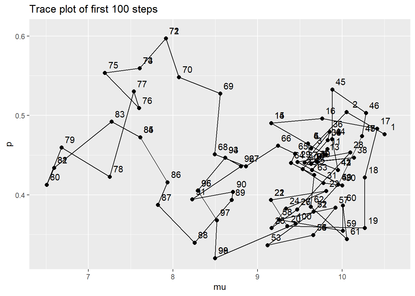

# Delete the first 1000 steps - we'll see why in the next chapter
theta = theta[-(1:1000), ]

ggplot(theta, aes(x = mu)) + 
 geom_histogram(aes(y=..density..), color = "black", fill = "white") +
 geom_density(size = 1, color = "seagreen")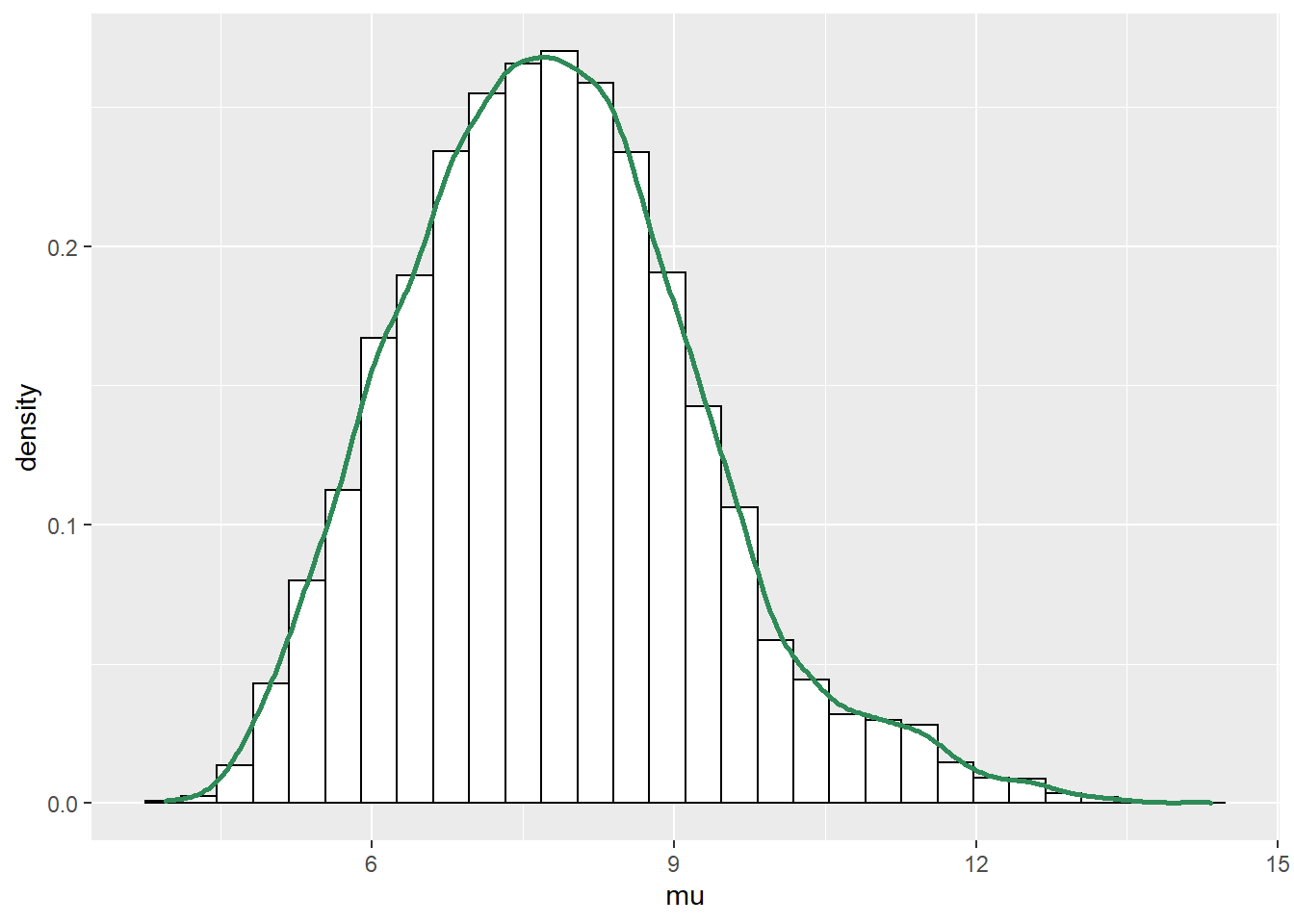

ggplot(theta, aes(x = p)) + 
 geom_histogram(aes(y=..density..), color = "black", fill = "white") +
 geom_density(size = 1, color = "seagreen")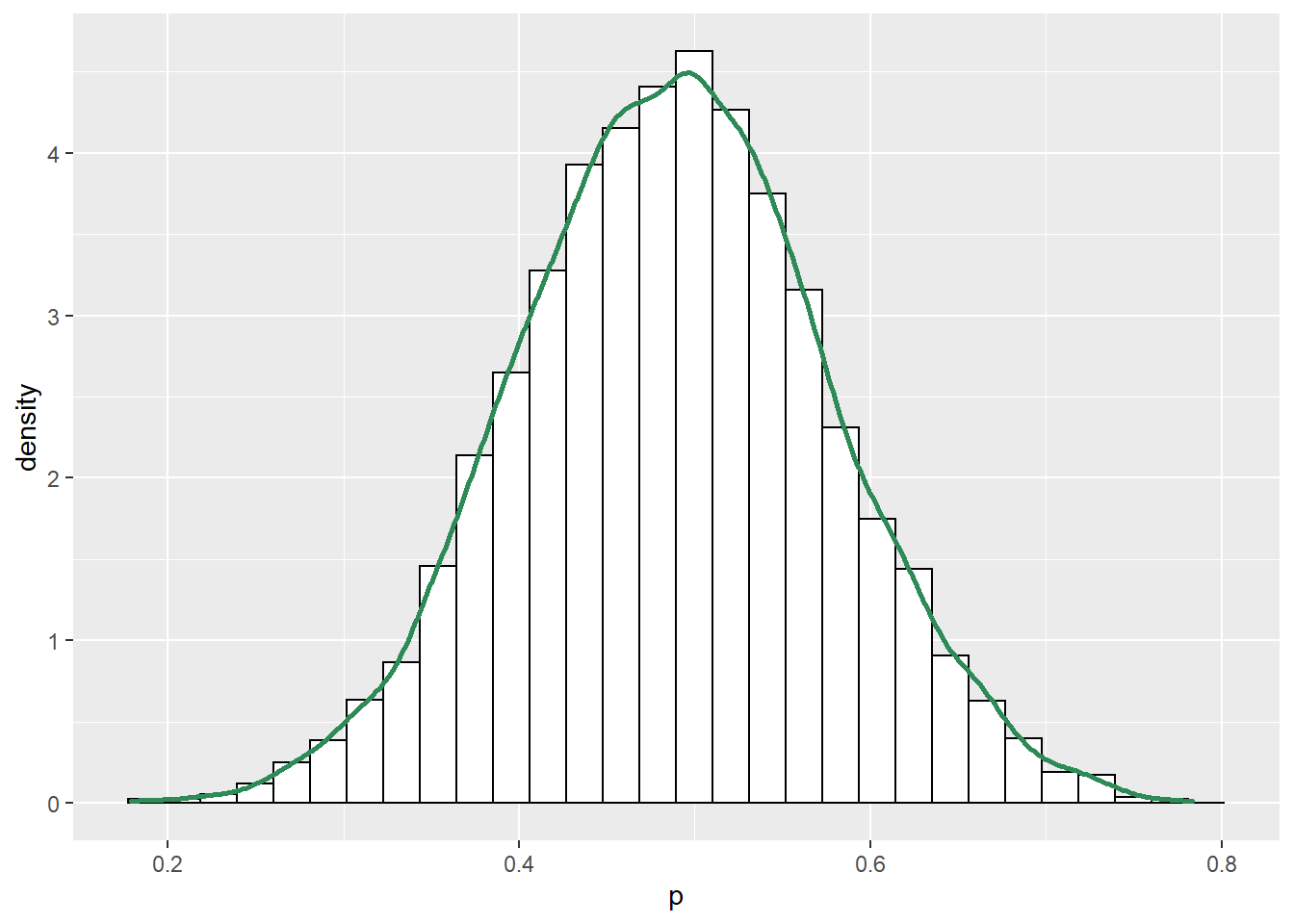

ggplot(theta, aes(mu, p)) +
  geom_point(color = "seagreen", alpha = 0.4) +
  stat_ellipse(level = 0.98, color = "black", size = 2) +
  stat_density_2d(color = "grey", size = 1) +
  geom_abline(intercept = 0, slope = 1)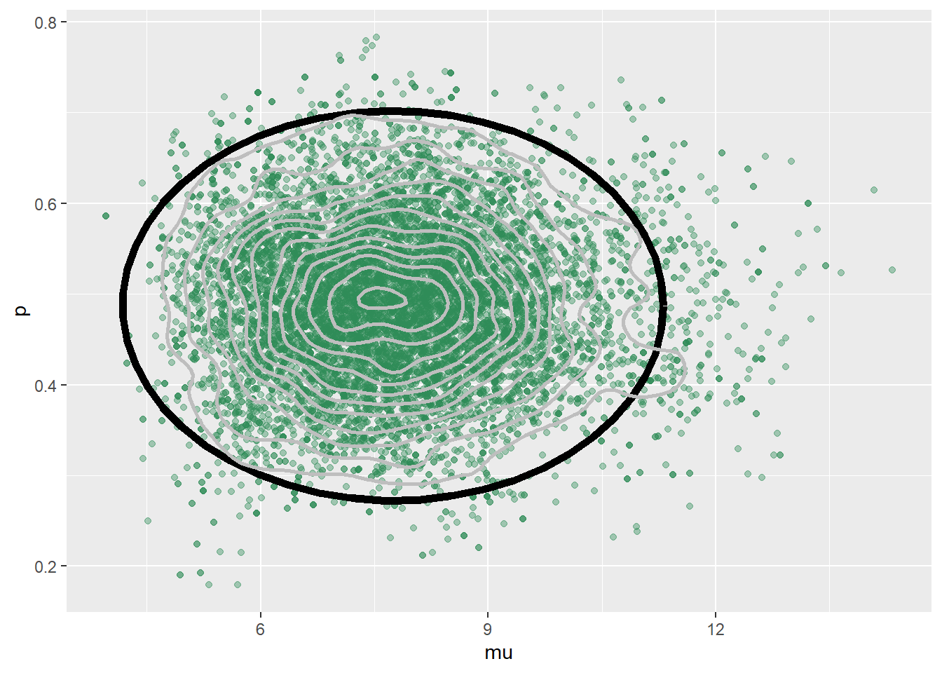

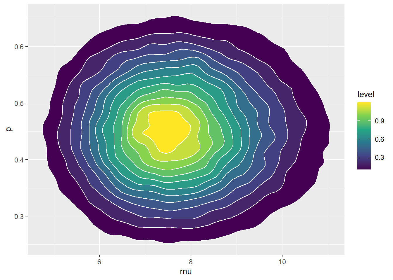
ggplot(theta, aes(mu, p)) +
  stat_density_2d(aes(fill = ..level..),
              geom = "polygon", color = "white") +
  scale_fill_viridis_c() +
  geom_abline(intercept = 0, slope = 1)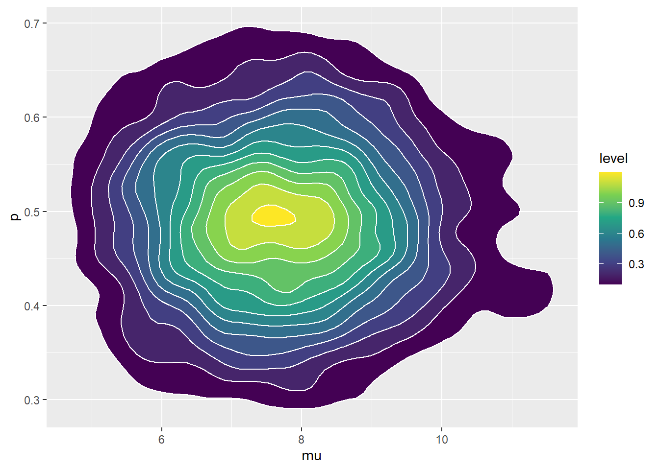

The JAGS code is below. The results are similar, but not quite the same as our code from scratch in the previous part. JAGS has a lot of built in features that improve efficiency. In particular, JAGS is making smarter proposals and is not rejecting as many proposals as our from-scratch algorithm. The scatterplots of simulated \((\mu, p)\) pairs kind of show this; the plot based on the from-scratch algorithm is “thinner” than the one based on JAGS because the from-scratch algorithm rejects proposals and sits in place more often.

# data
n = c(10, 11)
y = c(4, 6)
n_sample = 2


# Model
model_string <- "model{

  # Likelihood
  for (i in 1:n_sample){

  y[i] ~ dbinom(p, n[i])

  n[i] ~ dpois(mu)
  }

  # Prior

  mu ~ dgamma(10, 2)

  p ~ dbeta(4, 6)

}"

dataList = list(y = y, n = n, n_sample = n_sample)

# Compile
Nrep = 10000

n.chains = 5

model <- jags.model(textConnection(model_string),
                data = dataList,
                n.chains = n.chains)

## Compiling model graph
##    Resolving undeclared variables
##    Allocating nodes
## Graph information:
##    Observed stochastic nodes: 4
##    Unobserved stochastic nodes: 2
##    Total graph size: 11
## 
## Initializing model

# Simulate
update(model, 1000, progress.bar = "none")

posterior_sample <- coda.samples(model,
                             variable.names = c("mu", "p"),
                             n.iter = Nrep,
                             progress.bar = "none")

sim_posterior = as.data.frame(as.matrix(posterior_sample))
head(sim_posterior)

##       mu      p
## 1 10.904 0.5090
## 2  8.770 0.5579
## 3  8.269 0.4394
## 4  8.940 0.2968
## 5  7.712 0.3261
## 6  5.363 0.3156

ggplot(sim_posterior, aes(x = mu)) + 
 geom_histogram(aes(y=..density..), color = "black", fill = "white") +
 geom_density(size = 1, color = "seagreen")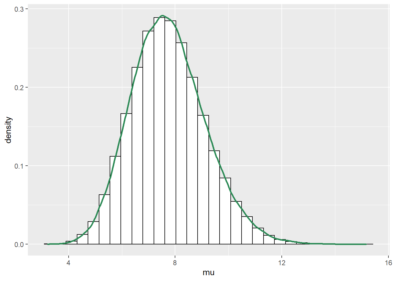

ggplot(sim_posterior, aes(x = p)) + 
 geom_histogram(aes(y=..density..), color = "black", fill = "white") +
 geom_density(size = 1, color = "seagreen")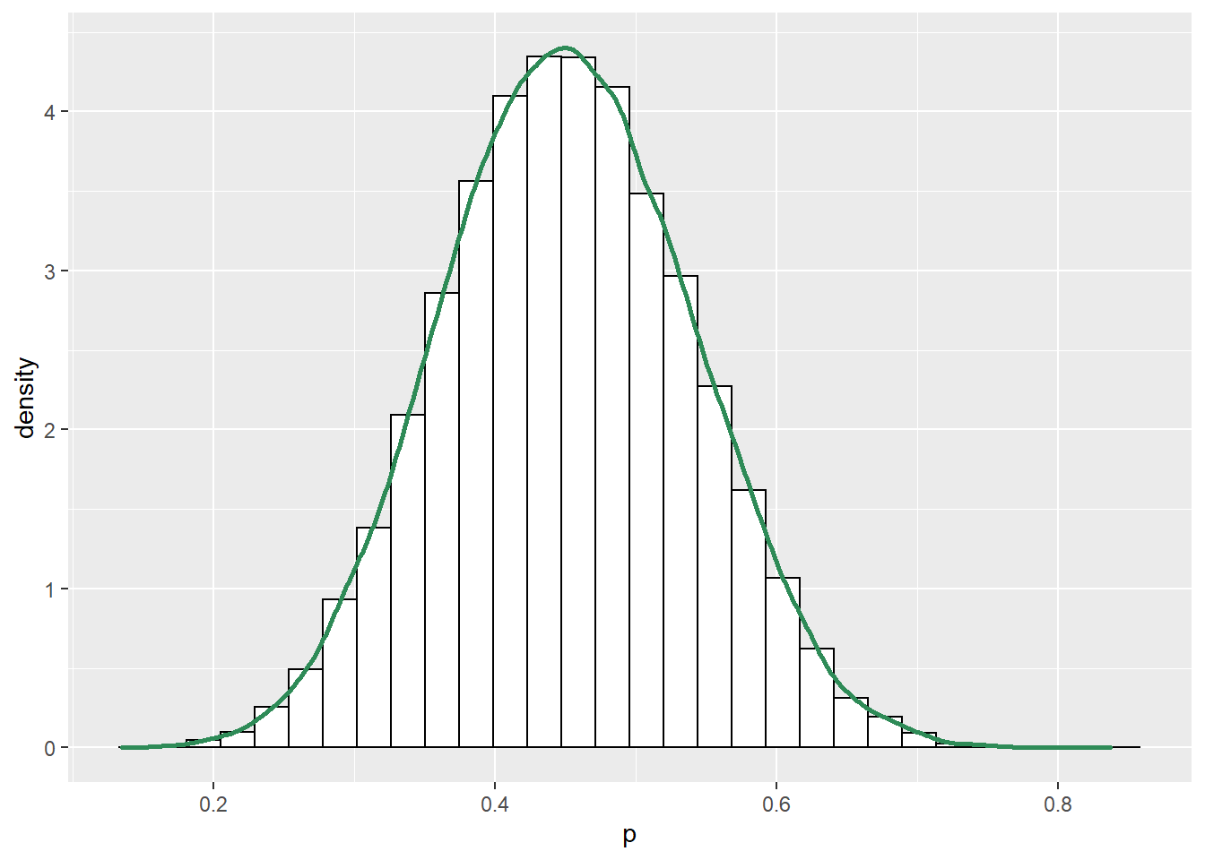

ggplot(sim_posterior, aes(mu, p)) +
  geom_point(color = "seagreen", alpha = 0.4) +
  stat_ellipse(level = 0.98, color = "black", size = 2) +
  stat_density_2d(color = "grey", size = 1) +
  geom_abline(intercept = 0, slope = 1)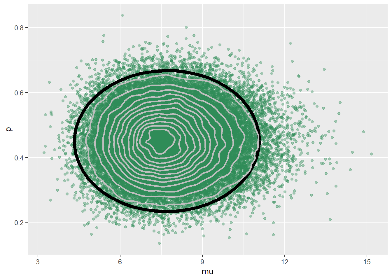

ggplot(sim_posterior, aes(mu, p)) +
  stat_density_2d(aes(fill = ..level..),
          geom = "polygon", color = "white") +
 scale_fill_viridis_c() +
  geom_abline(intercept = 0, slope = 1)