Chapter 13 Bayesian Analysis of Poisson Count Data
In this chapter we’ll consider Bayesian analysis for count data.
We have covered in some detail the problem of estimating a population proportion for a binary categorical variable. In these situations we assumed a Binomial likelihood for the count of “successes” in the sample. However, a Binomial model has several restrictive assumptions that might not be satisfied in practice. Poisson models are more flexible models for count data.
- In what ways is this like the Binomial situation? (What is a trial? What is “success”?)
- In what ways is this NOT like the Binomial situation?
Show/hide solution
- Each pitch is a trial, and on each trial either a home run is hit (“success”) or not. The random variable \(Y\) counts the number of home runs (successes) over all the trials
- Even though \(Y\) is counting successes, this is not the Binomial situation.
- The number of trials is not fixed. The total number of pitches varies from game to game. (The average is around 300 pitches per game).
- The probability of success is not the same on each trial. Different batters have different probabilities of hitting home runs. Also, different pitch counts or game situations lead to different probabilities of home runs.
- The trials might not be independent, though this is a little more questionable. Make sure you distinguish independence from the previous assumption of unequal probabilities of success; you need to consider conditional probabilities to assess independence. Maybe if a pitcher gives up a home run on one pitch, then the pitcher is “rattled” so the probability that he also gives up a home run on the next pitch increases, or the pitcher gets pulled for a new pitcher which changes the probability of a home run on the next pitch.
- In what ways is this like the Binomial situation? (What is a trial? What is “success”?)
- In what ways is this NOT like the Binomial situation?
Show/hide solution
- Each automobile on the road in the day is a trial, and on each automobile either gets in an accident (“success”) or not. The random variable \(Y\) counts the number of automobiles that get into accidents (successes). (Remember “success” is just a generic label for the event you’re interested in; “success” is not necessarily good.)
- Even though \(Y\) is counting successes, this is not the Binomial situation.
- The number of trials is not fixed. The total number of automobiles on the road varies from day to day.
- The probability of success is not the same on each trial. Different drivers have different probabilities of getting into accidents; some drivers are safer than others. Also, different conditions increase the probability of an accident, like driving at night.
- The trials are plausibly not independent. Make sure you distinguish independence from the previous assumption of unequal probabilities of success; you need to consider conditional probabilities to assess independence. If an automobile gets into an accident, then the probability of getting into an accident increases for the automobiles that are driving near it.
Poisson models are models for counts that have more flexibility than Binomial models. Poisson models are parameterized by a single parameter (the mean) and do not require all the assumptions of a Binomial model. Poisson distributions are often used to model the distribution of variables that count the number of “relatively rare” events that occur over a certain interval of time or in a certain location (e.g., number of accidents on a highway in a day, number of car insurance policies that have claims in a week, number of bank loans that go into default, number of mutations in a DNA sequence, number of earthquakes that occur in SoCal in an hour, etc.)
A discrete random variable \(Y\) has a Poisson distribution with parameter \(\theta>0\) if its probability mass function satisfies \[\begin{align*} f(y|\theta) & = \frac{e^{-\theta}\theta^y}{y!}, \quad y=0,1,2,\ldots \end{align*}\] If \(Y\) has a Poisson(\(\theta\)) distribution then \[\begin{align*} E(Y) & = \theta\\ Var(Y) & = \theta \end{align*}\]
For a Poisson distribution, both the mean and variance are equal to \(\theta\), but remember that the mean is measured in the count units (e.g., home runs) but the variance is measured in squared units (e.g., \((\text{home runs})^2\)).
Poisson distributions have many nice properties, including the following.
Poisson aggregation. If \(Y_1\) and \(Y_2\) are independent, \(Y_1\) has a Poisson(\(\theta_1\)) distribution, and \(Y_2\) has a Poisson(\(\theta_2\)) distribution, then \(Y_1+Y_2\) has a Poisson(\(\theta_1+\theta_2\)) distribution21. That is, if independent component counts each follow a Poisson distribution then the total count also follows a Poisson distribution. Poisson aggregation extends naturally to more than two components. For example, if the number of babies born each day at a certain hospital follows a Poisson distribution — perhaps with different daily rates (e.g., higher for Friday than Saturday) — independently from day to day, then the number of babies born each week at the hospital also follows a Poisson distribution.
Sketch your prior distribution for \(\theta\) and describe its features. What are the possible values of \(\theta\)? Does \(\theta\) take values on a discrete or continuous scale?
Suppose \(Y\) represents a home run count for a single game. What are the possible values of \(Y\)? Does \(Y\) take values on a discrete or continuous scale?
We’ll start with a discrete prior for \(\theta\) to illustrate ideas.
\(\theta\) 0.5 1.5 2.5 3.5 4.5 Probability 0.13 0.45 0.28 0.11 0.03 Suppose a single game with 1 home run is observed. Find the posterior distribution of \(\theta\). In particular, how do you determine the likelihood column?
Now suppose a second game, with 3 home runs, is observed, independently of the first. Find the posterior distribution of \(\theta\) after observing these two games, using the posterior distribution from the previous part as the prior distribution in this part.
Now consider the original prior again. Find the posterior distribution of \(\theta\) after observing 1 home run in the first game and 3 home runs in the second, without the intermediate updating of the posterior after the first game. How does the likelihood column relate to the likelihood columns from the previous parts? How does the posterior distribution compare with the posterior distribution from the previous part?
Now consider the original prior again. Suppose that instead of observing the two individual values, we only observe that there is a total of 4 home runs in 2 games. Find the posterior distribution of \(\theta\). In particular, you do you determine the likelihood column? How does the likelihood column compare to the one from the previous part? How does posterior compare to the previous part?
Suppose we’ll observe a third game tomorrow. How could you find — both analytically and via simulation —the posterior predictive probability that this game has 0 home runs?
Now let’s consider a continuous prior distribution for \(\theta\) which satisfies \[ \pi(\theta) \propto \theta^{4 -1}e^{-2\theta}, \qquad \theta > 0 \] Use grid approximation to compute the posterior distribution of \(\theta\) given 1 home run in a single game. Plot the prior, (scaled) likelihood, and posterior. (Note: you will need to cut the grid off at some point. While \(\theta\) can take any value greater than 0, the interval [0, 8] accounts for 99.99% of the prior probability.)
Now let’s consider some real data. Assume home runs per game at Citizens Bank Park (Phillies!) follow a Poisson distribution with parameter \(\theta\). Assume that the prior distribution for \(\theta\) satisfies \[ \pi(\theta) \propto \theta^{4 -1}e^{-2\theta}, \qquad \theta > 0 \] The following summarizes data for the 2020 season22. There were 97 home runs in 32 games. Use grid approximation to compute the posterior distribution of \(\theta\) given the data. Be sure to specify the likelihood. Plot the prior, (scaled) likelihood, and posterior.
Home runs Number of games 0 0 1 8 2 8 3 5 4 4 5 3 6 2 7 1 8 1 9 0 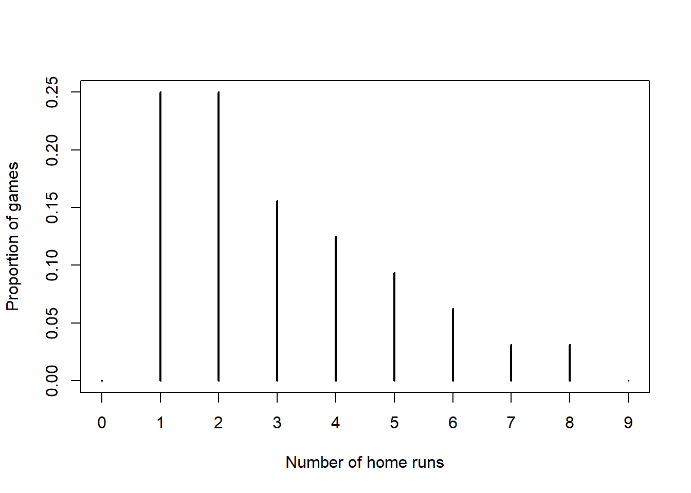
Your prior is whatever it is. We’ll discuss how we chose a prior in a later part. Even though each data value is an integer, the mean number of home runs per game \(\theta\) can be any value greater than 0. That is, the parameter \(\theta\) takes values on a continuous scale.
\(Y\) can be 0, 1, 2, and so on, taking values on a discrete scale. Technically, there is no fixed upper bound on what \(Y\) can be.
The likelihood is the Poisson probability of 1 home run in a game computed for each value of \(\theta\). \[ f(y=1|\theta) = \frac{e^{-\theta}\theta^1}{1!} \] For example, the likelihood of 1 home run in a game given \(\theta=0.5\) is \(f(y=1|\theta=0.5) = \frac{e^{-0.5}0.5^1}{1!} = 0.3033\). If on average there are 0.5 home runs per game, then about 30% of games would have exactly 1 home run. As always posterior is proportional to the product of prior and likelihood. We see that the posterior distibution puts even greater probability on \(\theta=1.5\) than the prior.
theta prior likelihood product posterior 0.5 0.13 0.3033 0.0394 0.1513 1.5 0.45 0.3347 0.1506 0.5779 2.5 0.28 0.2052 0.0575 0.2205 3.5 0.11 0.1057 0.0116 0.0446 4.5 0.03 0.0500 0.0015 0.0058 The likelihood is the Poisson probability of 3 home runs in a game computed for each value of \(\theta\). \[ f(y=3|\theta) = \frac{e^{-\theta}\theta^3}{3!} \]
The posterior places about 90% of the probability on \(\theta\) being either 1.5 or 2.5.
theta prior likelihood product posterior 0.5 0.1513 0.0126 0.0019 0.0145 1.5 0.5779 0.1255 0.0725 0.5488 2.5 0.2205 0.2138 0.0471 0.3566 3.5 0.0446 0.2158 0.0096 0.0728 4.5 0.0058 0.1687 0.0010 0.0073 Since the games are independent23 the likelihood is the product of the likelihoods from the two previous parts \[ f(y=(1, 3)|\theta) = \left(\frac{e^{-\theta}\theta^1}{1!}\right)\left(\frac{e^{-\theta}\theta^3}{3!}\right) \]
Unsuprisingly, the posterior distribution is the same as in the previous part.
theta prior likelihood product posterior 0.5 0.13 0.0038 0.0005 0.0145 1.5 0.45 0.0420 0.0189 0.5488 2.5 0.28 0.0439 0.0123 0.3566 3.5 0.11 0.0228 0.0025 0.0728 4.5 0.03 0.0084 0.0003 0.0073 By Poisson aggregation, the total number of home runs in 2 games follows a Poisson(\(2\theta\)) distribution. The likelihood is the probability of a value of 4 (home runs in 2 games) computed using a Poisson(\(2\theta\)) for each value of \(\theta\). \[ f(\bar{y}=2|\theta) = \frac{e^{-2\theta}(2\theta)^4}{4!} \] For example, the likelihood of 4 home runs in 2 games given \(\theta=0.5\) is \(f(\bar{y}=2|\theta=0.5) = \frac{e^{-2\times 0.5}(2\times 0.5)^4}{4!} = 0.0153\). If on average there are 0.5 home runs per game, then about 1.5% of samples of 2 games would have exactly 4 home runs.
The likelihood is not the same as in the previous part because there are more samples of two games that yield a total of 4 home runs than those that yield 1 home run in the first game and 3 in the second. However, the likelihoods are proportionally the same. For example, the likelihood for \(\theta=2.5\) is about 1.92 times greater than the likelihood for \(\theta = 3.5\) in both this part and the previous part. Therefore, the posterior distribution is the same as in the previous part.
theta prior likelihood product posterior 0.5 0.13 0.0153 0.0020 0.0145 1.5 0.45 0.1680 0.0756 0.5488 2.5 0.28 0.1755 0.0491 0.3566 3.5 0.11 0.0912 0.0100 0.0728 4.5 0.03 0.0337 0.0010 0.0073 Simulate a value of \(\theta\) from its posterior distribution and then given \(\theta\) simulate a value of \(Y\) from a Poisson(\(\theta\)) distribution, and repeat many times. Approximate the probability of 0 home runs by finding the proportion of repetitions that yield a \(Y\) value of 0. (We’ll see some code a little later.)
We can compute the probability using the law of total probability. Find the probability of 0 home runs for each value of \(\theta\), that is \(e^{-\theta}\theta^0/0! = e^{-\theta}\), and then weight these values by their posterior probabilities to find the predictive probability of 0 home runs, which is 0.163.
\[\begin{align*} & e^{-0.5}(0.0145) + e^{-1.5}(0.5488) + e^{-2.5}(0.3566) + e^{-3.5}(0.0728) + e^{-4.5}(0.0073)\\ = & (0.6065)(0.0145) + (0.2231)(0.5488) + (0.0821)(0.3566) + (0.0302)(0.0728) + (0.0111)(0.0073) = 0.1628 \end{align*}\]
According to this model, we predict that about 16% of games would have 0 home runs.
Now let’s consider a continuous prior distribution for \(\theta\) which satisfies \[ \pi(\theta) \propto \theta^{4 -1}e^{-2\theta}, \qquad \theta > 0 \] Use grid approximation to compute the posterior distribution of \(\theta\) given 1 home run in a single game. Plot the prior, (scaled) likelihood, and posterior. (Note: you will need to cut the grid off at some point. While \(\theta\) can take any value greater than 0, the interval [0, 8] accounts for 99.99% of the prior probability.)
# prior
theta = seq(0, 8, 0.001)

prior = theta ^ (4 - 1) * exp(-2 * theta)
prior = prior / sum(prior)

# data
n = 1 # sample size
y = 1 # sample mean

# likelihood
likelihood = dpois(y, theta)

# posterior
product = likelihood * prior
posterior = product / sum(product)

ylim = c(0, max(c(prior, posterior, likelihood / sum(likelihood))))
xlim = range(theta)
plot(theta, prior, type='l', xlim=xlim, ylim=ylim, col="orange", xlab='theta', ylab='', yaxt='n')
par(new=T)
plot(theta, likelihood/sum(likelihood), type='l', xlim=xlim, ylim=ylim, col="skyblue", xlab='', ylab='', yaxt='n')
par(new=T)
plot(theta, posterior, type='l', xlim=xlim, ylim=ylim, col="seagreen", xlab='', ylab='', yaxt='n')
legend("topright", c("prior", "scaled likelihood", "posterior"), lty=1, col=c("orange", "skyblue", "seagreen"))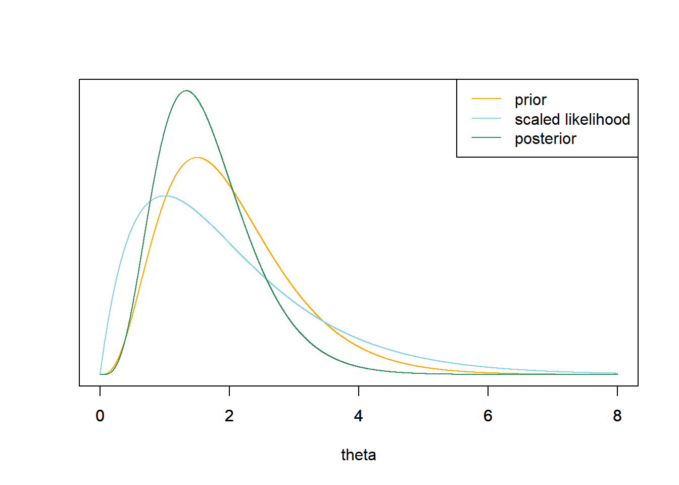
By Poisson aggregation, the total number of home runs in 32 games follows a Poisson(\(32\theta\)) distribution. The likelihood is the probability of observing a value of 97 (for the total number of home runs in 32 games) from a Poisson(\(32\theta\)) distribution. \[\begin{align*} f(\bar{y} = 97/32|\theta) & = e^{-32\theta}(32\theta)^{97}/97!, \qquad \theta > 0\\ & \propto e^{-32\theta}\theta^{97}, \qquad \theta > 0\\ \end{align*}\]
The likelihood is centered at the sample mean of 97/32 = 3.03. The posterior distribution follows the likelihood fairly closely, but the prior still has a little influence.
# prior
theta = seq(0, 8, 0.001)

prior = theta ^ (4 - 1) * exp(-2 * theta)
prior = prior / sum(prior)

# data
n = 32 # sample size
y = 97 / 32 # sample mean

# likelihood - for total count
likelihood = dpois(n * y, n * theta)

# posterior
product = likelihood * prior
posterior = product / sum(product)

ylim = c(0, max(c(prior, posterior, likelihood / sum(likelihood))))
xlim = range(theta)
plot(theta, prior, type='l', xlim=xlim, ylim=ylim, col="orange", xlab='theta', ylab='', yaxt='n')
par(new=T)
plot(theta, likelihood/sum(likelihood), type='l', xlim=xlim, ylim=ylim, col="skyblue", xlab='', ylab='', yaxt='n')
par(new=T)
plot(theta, posterior, type='l', xlim=xlim, ylim=ylim, col="seagreen", xlab='', ylab='', yaxt='n')
legend("topright", c("prior", "scaled likelihood", "posterior"), lty=1, col=c("orange", "skyblue", "seagreen"))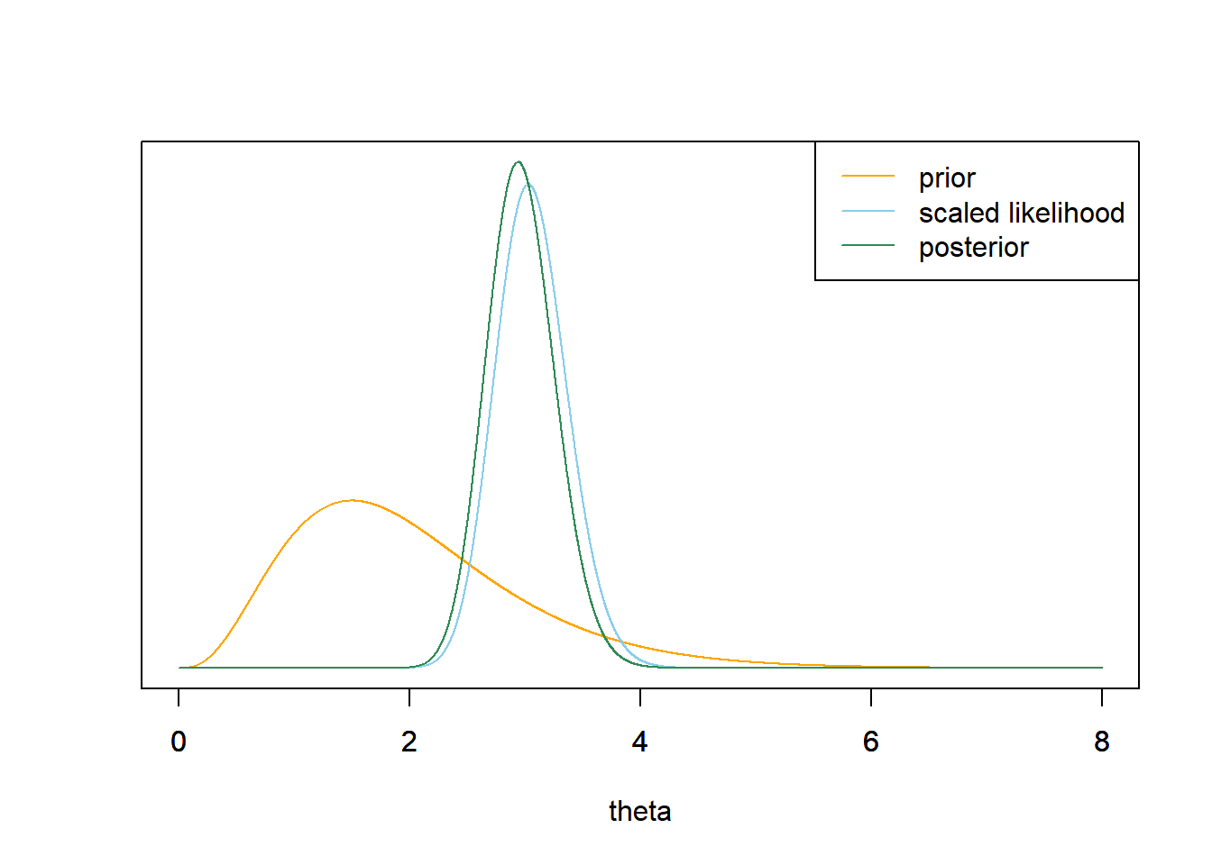
Gamma distributions are commonly used as prior distributions for parameters that take positive values, \(\theta > 0\).
A continuous RV \(U\) has a Gamma distribution with shape parameter \(\alpha>0\) and rate parameter24 \(\lambda>0\) if its density satisfies25 \[ f(u) \propto u^{\alpha-1}e^{-\lambda u}, \quad u>0, \]
In R: dgamma(u, shape, rate) for density, rgamma to simulate, qgamma for quantiles, etc.
It can be shown that a Gamma(\(\alpha\), \(\lambda\)) density has \[\begin{align*} \text{Mean (EV)} & = \frac{\alpha}{\lambda}\\ \text{Variance} & = \frac{\alpha}{\lambda^2} \\ \text{Mode} & = \frac{\alpha -1}{\lambda}, \qquad \text{if $\alpha\ge 1$} \end{align*}\]
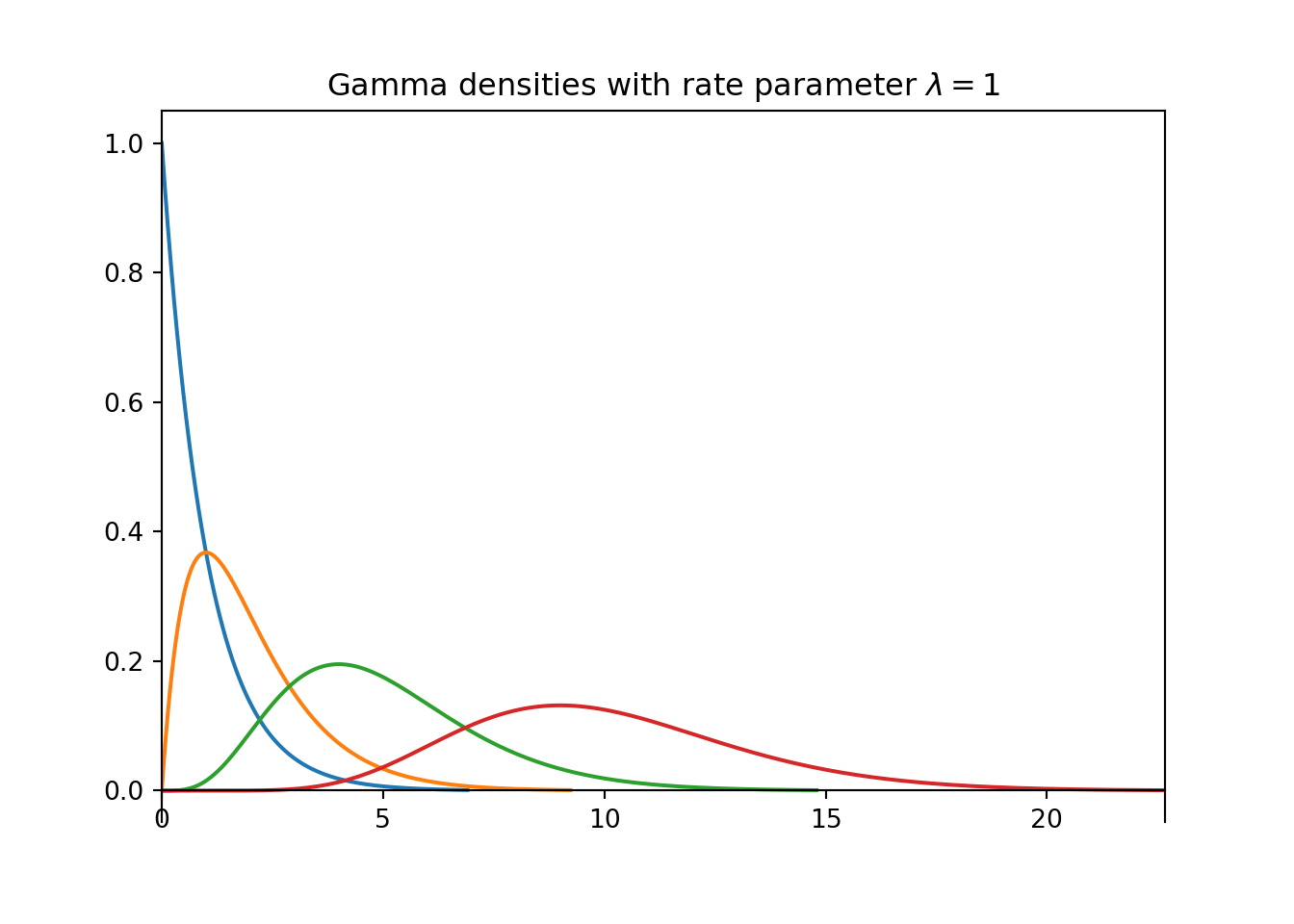
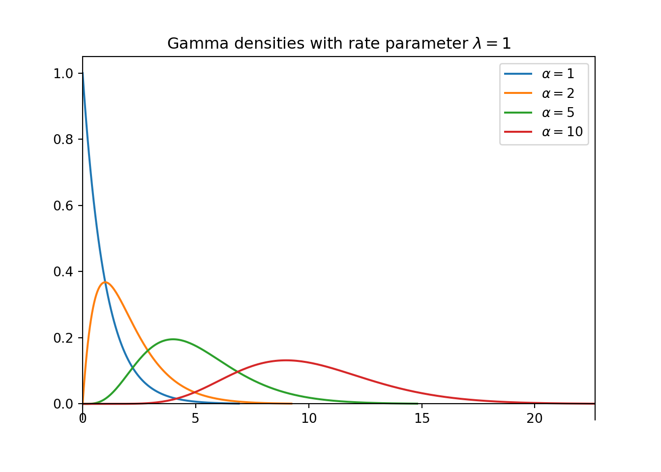
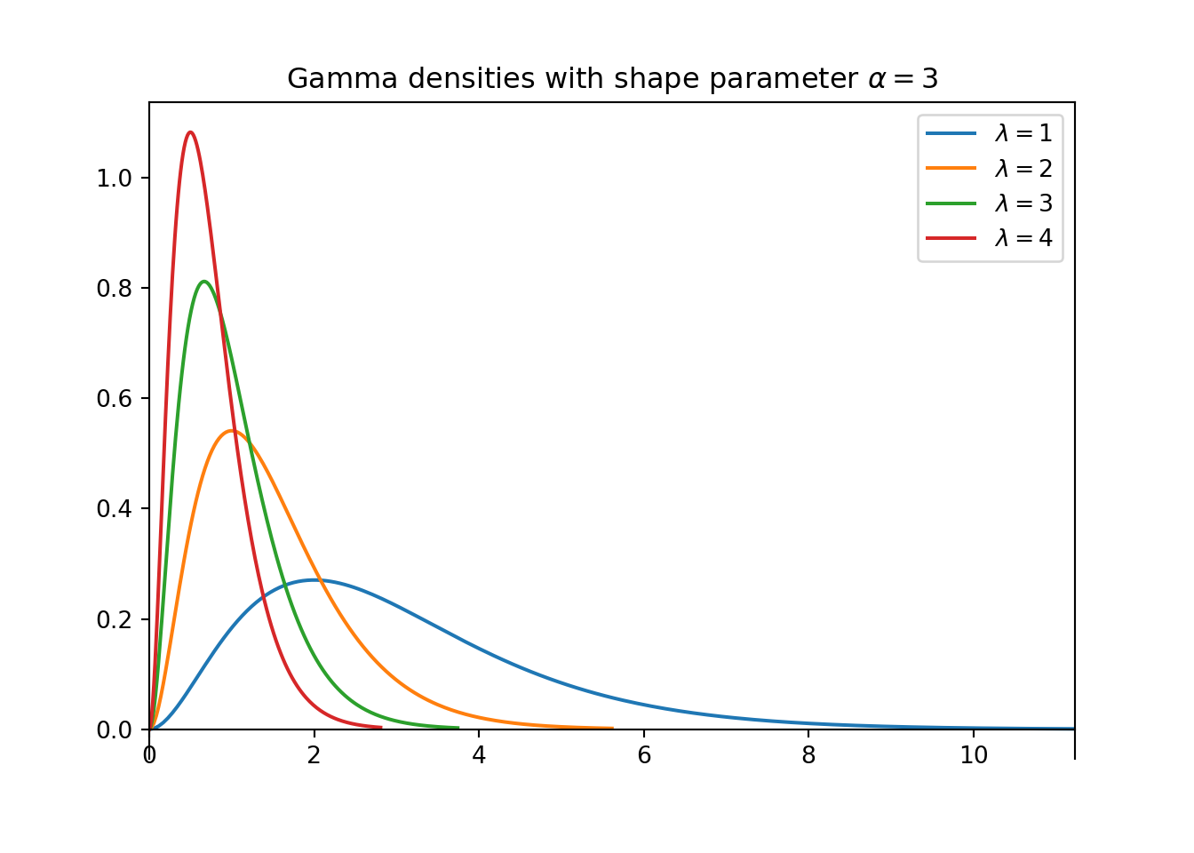
- The plot on the left above contains a few different Gamma densities, all with rate parameter \(\lambda=1\). Match each density to its shape parameter \(\alpha\); the choices are 1, 2, 5, 10.
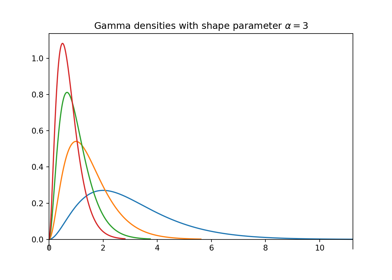
- The plot on the right above contains a few different Gamma densities, all with shape parameter \(\alpha=3\). Match each density to its rate parameter \(\lambda\); the choices are 1, 2, 3, 4.
For a fixed \(\lambda\), as the shape parameter \(\alpha\) increases, both the mean and the standard deviation increase.
For a fixed \(\alpha\), as the rate parameter \(\lambda\) increases, both the mean and the standard deviation decrease.
Observe that changing \(\lambda\) doesn’t change the overall shape of the curve, just the scale of values that it covers. However, changing \(\alpha\) does change the shape of the curve; notice the changes in concavity in the plot on the left.
- Write an expression for the prior density \(\pi(\theta)\). Plot the prior distribution. Find the prior mean, prior SD, and prior 50%, 80%, and 98% credible intervals for \(\theta\).
- Suppose a single game with 1 home run is observed. Write the likelihood function.
- Write an expression for the posterior distribution of \(\theta\) given a single game with 1 home run. Identify by the name the posterior distribution and the values of relevant parameters. Plot the prior distribution, (scaled) likelihood, and posterior distribution. Find the posterior mean, posterior SD, and posterior 50%, 80%, and 98% credible intervals for \(\theta\).
- Now consider the original prior again. Determine the likelihood of observing 1 home run in game 1 and 3 home runs in game 2 in a sample of 2 games, and the posterior distribution of \(\theta\) given this sample. Identify by the name the posterior distribution and the values of relevant parameters. Plot the prior distribution, (scaled) likelihood, and posterior distribution. Find the posterior mean, posterior SD, and posterior 50%, 80%, and 98% credible intervals for \(\theta\).
- Consider the original prior again. Determine the likelihood of observing a total of 4 home runs in a sample of 2 games, and the posterior distribution of \(\theta\) given this sample. Identify by the name the posterior distribution and the values of relevant parameters. How does this compare to the previous part?
- Consider the 2020 data in which there were 97 home runs in 32 games. Determine the likelihood function, and the posterior distribution of \(\theta\) given this sample. Identify by the name the posterior distribution and the values of relevant parameters. Plot the prior distribution, (scaled) likelihood, and posterior distribution. Find the posterior mean, posterior SD, and posterior 50%, 80%, and 98% credible intervals for \(\theta\).
- Interpret the credible interval from the previous part in context.
- Express the posterior mean of \(\theta\) based on the 2020 data as a weighted average of the prior mean and the sample mean.
- While the main parameter is \(\theta\), there are other parameters of interest. For example, \(\eta = e^{-\theta}\) is the population proportion of games in which there are 0 home runs. Assuming that you already have the posterior distribution of \(\theta\) (or a simulation-based approximation), explain how you could use simulation to approximate the posterior distribution of \(\eta\). Run the simulation and plot the posterior distribution, and find and interpret 50%, 80%, and 98% posterior credible intervals for \(\eta\).
- Use JAGS to approximate the posterior distribution of \(\theta\) given this sample. Compare with the results from the previous example.
Remember that in the Gamma(4,2) prior distribution \(\theta\) is treated as the variable. \[ \pi(\theta) \propto \theta^{4-1}e^{-2\theta}, \qquad \theta > 0. \]
This is the same prior we used in the grid approximation in Example 13.3. See below for a plot. \[\begin{align*} \text{Prior mean } & = \frac{\alpha}{\lambda} & & \frac{4}{2} = 2\\ \text{Prior SD} & = \sqrt{\frac{\alpha}{\lambda^2}} & & \sqrt{\frac{4}{2^2}} = 1 \end{align*}\]
Use
qgammafor find the endpoints of the credible intervals.qgamma(c(0.25, 0.75), shape = 4, rate = 2)## [1] 1.268 2.555qgamma(c(0.10, 0.90), shape = 4, rate = 2)## [1] 0.8724 3.3404qgamma(c(0.01, 0.99), shape = 4, rate = 2)## [1] 0.4116 5.0226The likelihood is the Poisson probability of 1 home run in a game computed for each value of \(\theta>0\). \[ f(y=1|\theta) = \frac{e^{-\theta}\theta^1}{1!}\propto e^{-\theta}\theta, \qquad \theta>0. \]
Posterior is proportional to likelihood times prior \[\begin{align*} \pi(\theta|y = 1) & \propto \left(e^{-\theta}\theta\right)\left(\theta^{4-1}e^{-2\theta}\right), \qquad \theta > 0,\\ & \propto \theta^{(4 + 1) - 1}e^{-(2+1)\theta}, \qquad \theta > 0. \end{align*}\]
We recognize the above as the Gamma density with shape parameter \(\alpha=4+1\) and rate parameter \(\lambda = 2 + 1\).
\[\begin{align*} \text{Posterior mean } & = \frac{\alpha}{\lambda} & & \frac{5}{3} = 1.667\\ \text{Posterior SD} & = \sqrt{\frac{\alpha}{\lambda^2}} & & \sqrt{\frac{5}{3^2}} = 0.745 \end{align*}\]
qgamma(c(0.25, 0.75), shape = 4 + 1, rate = 2 + 1)## [1] 1.123 2.091qgamma(c(0.10, 0.90), shape = 4 + 1, rate = 2 + 1)## [1] 0.8109 2.6645qgamma(c(0.01, 0.99), shape = 4 + 1, rate = 2 + 1)## [1] 0.4264 3.8682theta = seq(0, 8, 0.001) # the grid is just for plotting # prior alpha = 4 lambda = 2 prior = dgamma(theta, shape = alpha, rate = lambda) # likelihood n = 1 # sample size y = 1 # sample mean likelihood = dpois(n * y, n * theta) # posterior posterior = dgamma(theta, alpha + n * y, lambda + n) # plot plot_continuous_posterior <- function(theta, prior, likelihood, posterior) { ymax = max(c(prior, posterior)) scaled_likelihood = likelihood * ymax / max(likelihood) plot(theta, prior, type='l', col='orange', xlim= range(theta), ylim=c(0, ymax), ylab='', yaxt='n') par(new=T) plot(theta, scaled_likelihood, type='l', col='skyblue', xlim=range(theta), ylim=c(0, ymax), ylab='', yaxt='n') par(new=T) plot(theta, posterior, type='l', col='seagreen', xlim=range(theta), ylim=c(0, ymax), ylab='', yaxt='n') legend("topright", c("prior", "scaled likelihood", "posterior"), lty=1, col=c("orange", "skyblue", "seagreen")) } plot_continuous_posterior(theta, prior, likelihood, posterior)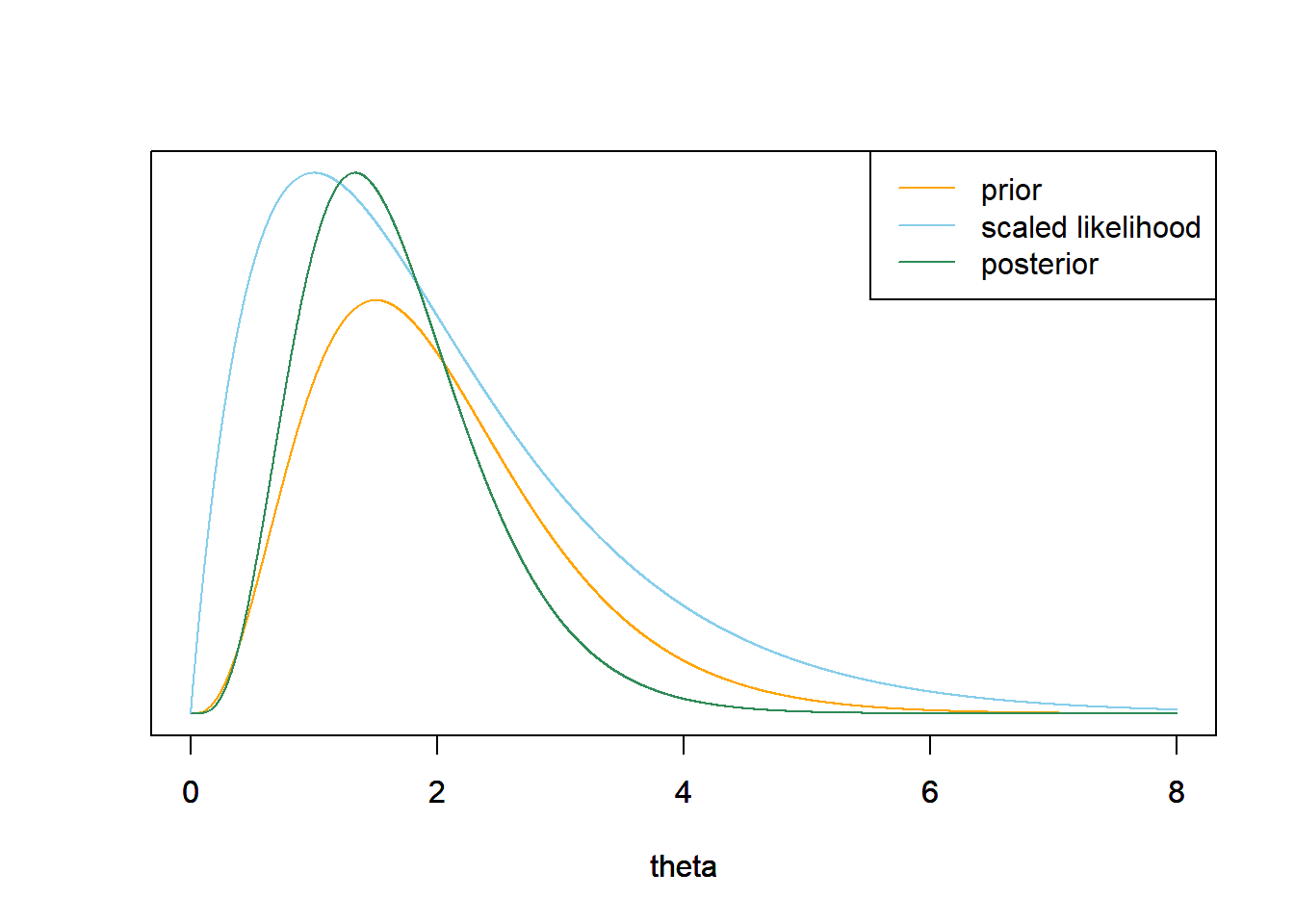
The likelihood is the product of the likelihoods of \(y=1\) and \(y=3\). \[ f(y=(1, 3)|\theta) = \left(\frac{e^{-\theta}\theta^1}{1!}\right)\left(\frac{e^{-\theta}\theta^3}{3!}\right) \propto e^{-2\theta}\theta^{4}, \qquad \theta>0. \]
The posterior satisfies \[\begin{align*} \pi(\theta|y = (1, 3)) & \propto \left(e^{-2\theta}\theta^4\right)\left(\theta^{4-1}e^{-2\theta}\right), \qquad \theta > 0,\\ & \propto \theta^{(4 + 4) - 1}e^{-(2+2)\theta}, \qquad \theta > 0. \end{align*}\]
We recognize the above as the Gamma density with shape parameter \(\alpha=4+4\) and rate parameter \(\lambda = 2 + 2\).
\[\begin{align*} \text{Posterior mean } & = \frac{\alpha}{\lambda} & & \frac{8}{4} = 2\\ \text{Posterior SD} & = \sqrt{\frac{\alpha}{\lambda^2}} & & \sqrt{\frac{8}{4^2}} = 0.707 \end{align*}\]
qgamma(c(0.25, 0.75), shape = 4 + 4, rate = 2 + 2)## [1] 1.489 2.421qgamma(c(0.10, 0.90), shape = 4 + 4, rate = 2 + 2)## [1] 1.164 2.943qgamma(c(0.01, 0.99), shape = 4 + 4, rate = 2 + 2)## [1] 0.7265 4.0000n = 2 # sample size y = 2 # sample mean # likelihood likelihood = dpois(1, theta) * dpois(3, theta) # posterior posterior = dgamma(theta, alpha + n * y, lambda + n) # plot plot_continuous_posterior(theta, prior, likelihood, posterior)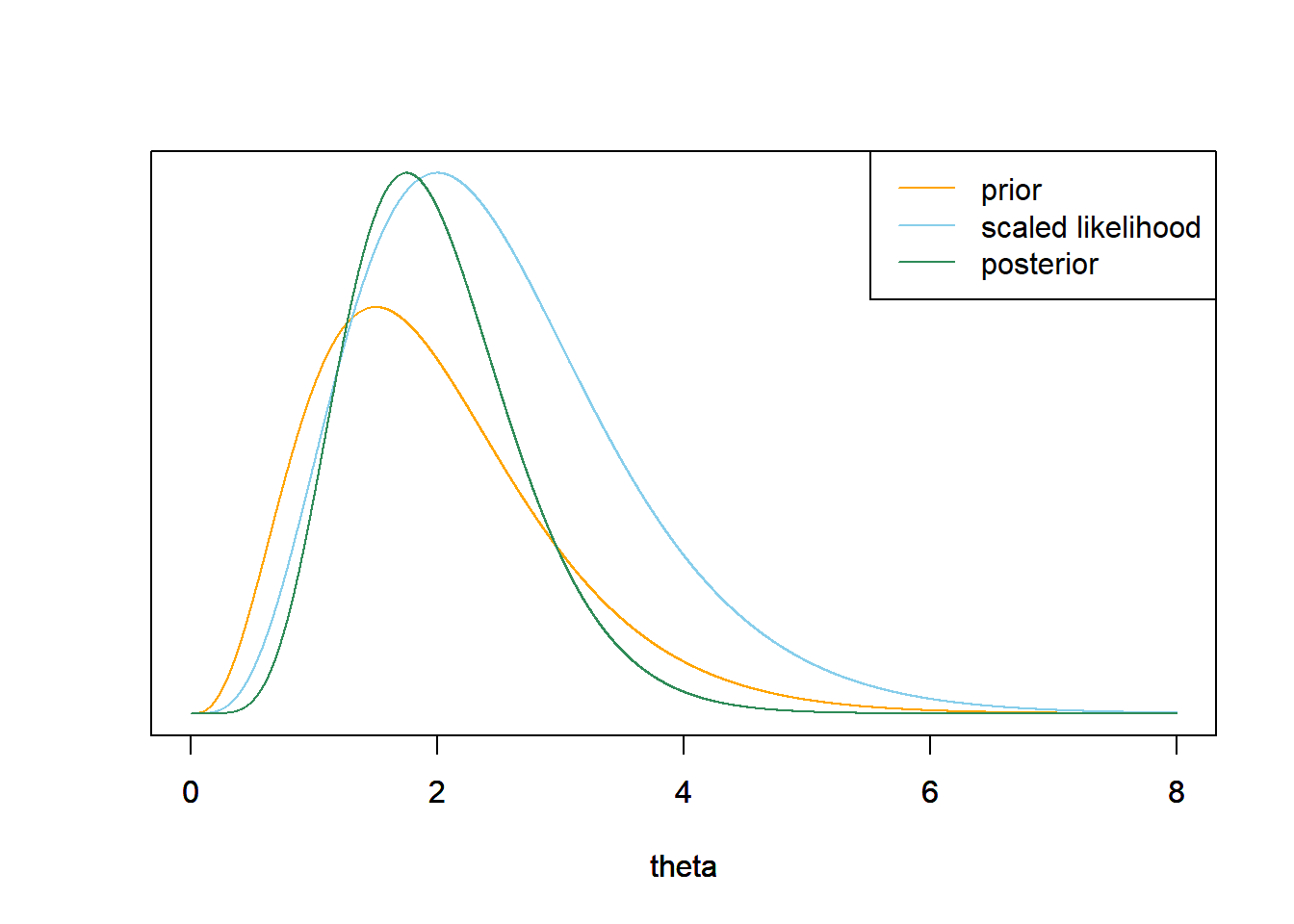
By Poisson aggregation, the total number of home runs in 2 games follows a Poisson(\(2\theta\)) distribution. The likelihood is the probability of a value of 4 (home runs in 2 games) computed using a Poisson(\(2\theta\)) for each value of \(\theta\). \[ f(\bar{y}=2|\theta) = \frac{e^{-2\theta}(2\theta)^4}{4!} \propto e^{-2\theta}\theta^4, \qquad \theta >0 \] The shape of the likelihood as a function of \(\theta\) is the same as in the previous part; the likelihood functions are proportionally the same regardless of whether you observe the individual values or just the total count. Therefore, the posterior distribution is the same as in the previous part.
# likelihood
n = 2 # sample size
y = 2 # sample mean
likelihood = dpois(n * y, n * theta)

# posterior
posterior = dgamma(theta, alpha + n * y, lambda + n)

# plot
plot_continuous_posterior(theta, prior, likelihood, posterior)
By Poisson aggregation, the total number of home runs in 32 games follows a Poisson(\(32\theta\)) distribution. The likelihood is the probability of observing a value of 97 (for the total number of home runs in 32 games) from a Poisson(\(32\theta\)) distribution. \[\begin{align*} f(\bar{y} = 97/32|\theta) & = e^{-32\theta}(32\theta)^{97}/97!, \qquad \theta > 0\\ & \propto e^{-32\theta}\theta^{97}, \qquad \theta > 0\\ \end{align*}\]
The posterior satisfies \[\begin{align*} \pi(\theta|\bar{y} = 97/32) & \propto \left(e^{-32\theta}\theta^{97}\right)\left(\theta^{4-1}e^{-2\theta}\right), \qquad \theta > 0,\\ & \propto \theta^{(4 + 97) - 1}e^{-(2+32)\theta}, \qquad \theta > 0. \end{align*}\]
We recognize the above as the Gamma density with shape parameter \(\alpha=4+97\) and rate parameter \(\lambda = 2 + 32\).
\[\begin{align*} \text{Posterior mean } & = \frac{\alpha}{\lambda} & & \frac{101}{34} = 2.97\\ \text{Posterior SD} & = \sqrt{\frac{\alpha}{\lambda^2}} & & \sqrt{\frac{101}{34^2}} = 0.296 \end{align*}\]
The likelihood is centered at the sample mean of 97/32 = 3.03. The posterior distribution follows the likelihood fairly closely, but the prior still has a little influence. The posterior is essentially identical to the one we computed via grid approximation in Example 13.3.
# likelihood
n = 32 # sample size
y = 97 / 32 # sample mean
likelihood = dpois(n * y, n * theta)

# posterior
posterior = dgamma(theta, alpha + n * y, lambda + n)

# plot
plot_continuous_posterior(theta, prior, likelihood, posterior)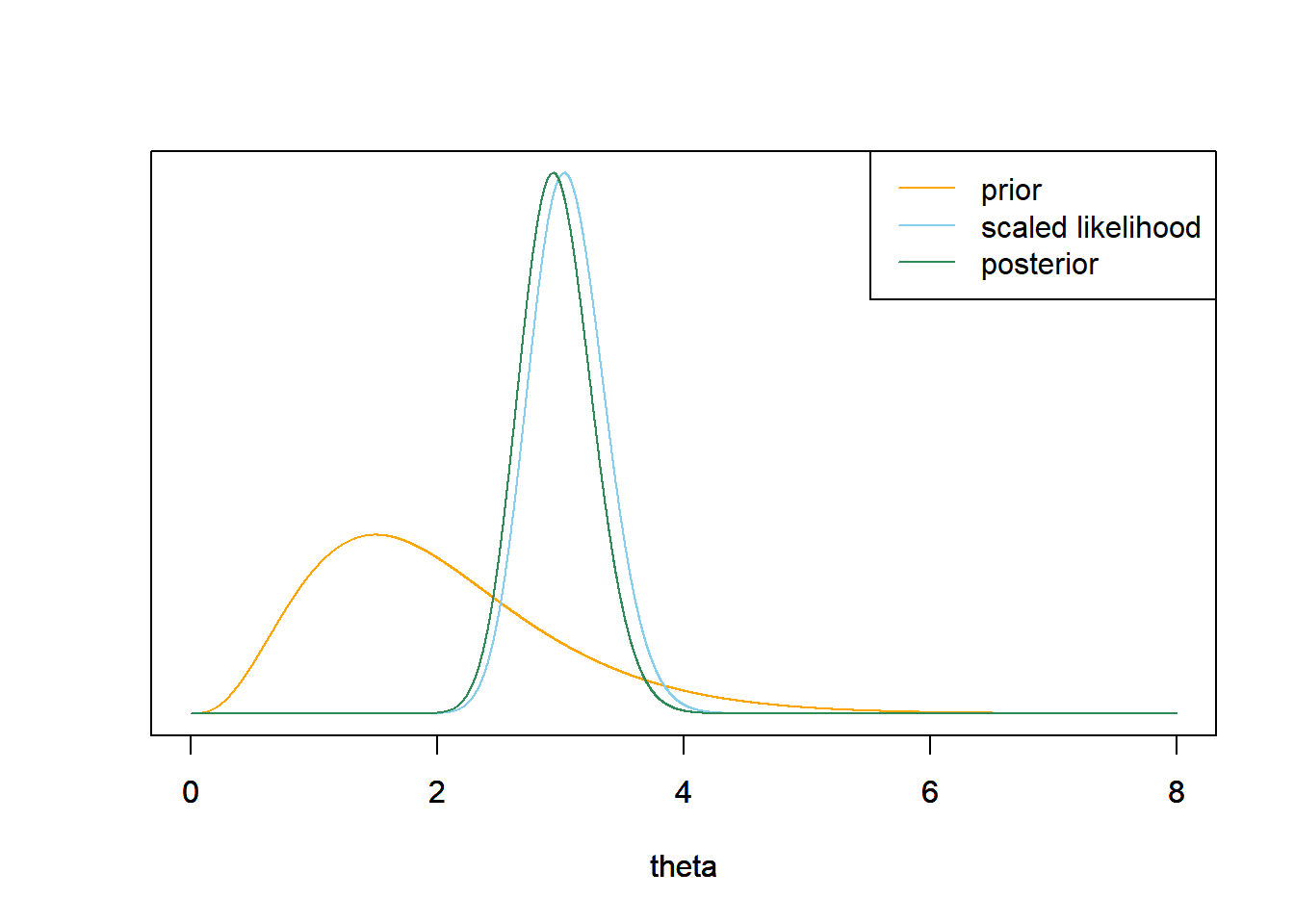
qgamma(c(0.25, 0.75), alpha + n * y, lambda + n)## [1] 2.766 3.164qgamma(c(0.10, 0.90), alpha + n * y, lambda + n)## [1] 2.599 3.355qgamma(c(0.01, 0.99), alpha + n * y, lambda + n)## [1] 2.326 3.701The credible intervals represent conclusions about \(\theta\), the mean number of home runs per game at Citizen Bank Park.
There is a posterior probability of 50% that the mean number of home runs per games at Citizen Bank Park is between 2.77 and 3.16. It is equally plausible that \(\theta\) is inside this interval as outside.
There is a posterior probability of 80% that the mean number of home runs per games at Citizen Bank Park is between 2.6 and 3.36. It is four times more plausible that \(\theta\) is inside this interval than outside.
There is a posterior probability of 98% that the mean number of home runs per games at Citizen Bank Park is between 2.33 and 3.7. It is 49 times more plausible that \(\theta\) is inside this interval than outside.
The prior mean is 4/2=2, based on a “prior sample size” of 2. The sample mean is 97/32 = 3.03, based on a sample size of 32. The posterior mean is (4 + 97)/(2 + 32) = 2.97. The posterior mean is a weighted average of the prior mean and the sample mean with the weights based on the “sample sizes” \[ 2.97 = \frac{4+97}{2 + 32} = \left(\frac{2}{2 + 32}\right)\left(\frac{4}{2}\right) + \left(\frac{32}{2 + 32}\right)\left(\frac{97}{32}\right) = (0.0589)(2)+ (0.941)(3.03) \]
Simulate a value of \(\theta\) from its posterior distribution, compute \(\eta = e^{-\theta}\), repeat many times, and summarize the simulated values of \(\eta\). We can use the
quantilefunction to find the endpoints of credible intervals.theta_sim = rgamma(10000, alpha + n * y, lambda + n) eta_sim = exp(-theta_sim) hist(eta_sim, freq = FALSE, xlab = "Population proportion of games with 0 HRs", ylab = "Posterior density", main = "Posterior distribution of exp(-theta)")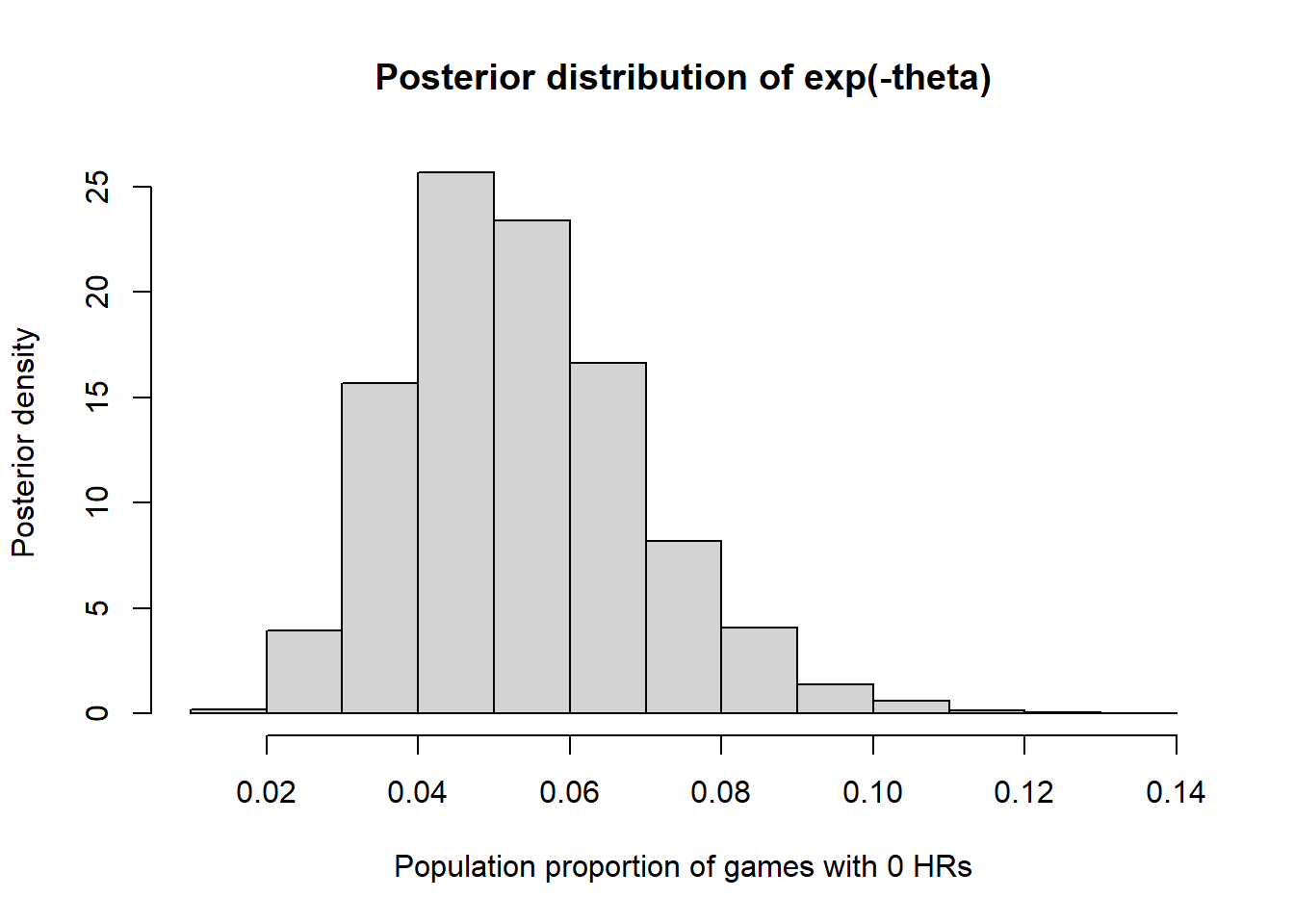
quantile(eta_sim, c(0.25, 0.75))## 25% 75% ## 0.04220 0.06315quantile(eta_sim, c(0.10, 0.90))## 10% 90% ## 0.03481 0.07455quantile(eta_sim, c(0.01, 0.99))## 1% 99% ## 0.02488 0.09849There is a posterior probability of 98% that the population proportion of games with 0 home runs is between 0.025 and 0.098.
The JAGS code is below. The results are very similar to the theoretical results from previous parts.
Here is the JAGS code. Note
- The data has been loaded as individual values, number of home runs in each of the 32 games
- Likelihood is defined as a loop. For each
y[i]value, the likelihood is computing according to a Poisson(\(\theta\)) distribution - Prior distribution is a Gamma distribution. (Remember, JAGS syntax for
dgamma,dpois, etc, is not the same as in R.)
# data
df = read.csv("_data/citizens-bank-hr-2020.csv")
y = df$hr
n = length(y)

# model
model_string <- "model{

  # Likelihood
  for (i in 1:n){
    y[i] ~ dpois(theta)
  }

  # Prior
  theta ~ dgamma(alpha, lambda)
  alpha <- 4
  lambda <- 2

}"

# Compile the model
dataList = list(y=y, n=n)

Nrep = 10000
Nchains = 3

model <- jags.model(textConnection(model_string),
                    data=dataList,
                    n.chains=Nchains)
## Compiling model graph
## Resolving undeclared variables
## Allocating nodes
## Graph information:
## Observed stochastic nodes: 32
## Unobserved stochastic nodes: 1
## Total graph size: 36
##
## Initializing modelupdate(model, 1000, progress.bar="none")
posterior_sample <- coda.samples(model,
variable.names=c("theta"),
n.iter=Nrep,
progress.bar="none")
# Summarize and check diagnostics
summary(posterior_sample)##
## Iterations = 1001:11000
## Thinning interval = 1
## Number of chains = 3
## Sample size per chain = 10000
##
## 1. Empirical mean and standard deviation for each variable,
## plus standard error of the mean:
##
## Mean SD Naive SE Time-series SE
## 2.96841 0.29380 0.00170 0.00171
##
## 2. Quantiles for each variable:
##
## 2.5% 25% 50% 75% 97.5%
## 2.42 2.77 2.96 3.16 3.57plot(posterior_sample)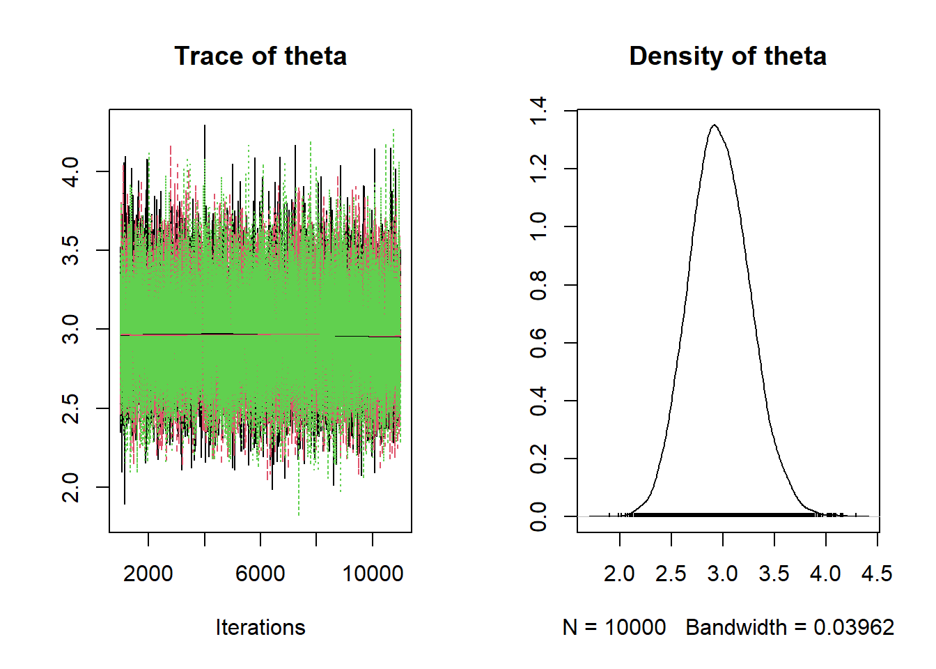
In the previous example we saw that if the values of the measured variable follow a Poisson distribution with parameter \(\theta\) and the prior for \(\theta\) follows a Gamma distribution, then the posterior distribution for \(\theta\) given the data also follows a Gamma distribution.
Gamma-Poisson model.26 Consider a measured variable \(Y\) which, given \(\theta\), follows a Poisson\((\theta)\) distribution. Let \(\bar{y}\) be the sample mean for a random sample of size \(n\). Suppose \(\theta\) has a Gamma\((\alpha, \lambda)\) prior distribution. Then the posterior distribution of \(\theta\) given \(\bar{y}\) is the Gamma\((\alpha+n\bar{y}, \lambda+n)\) distribution.
That is, Gamma distributions form a conjugate prior family for a Poisson likelihood.
The posterior distribution is a compromise between prior and likelihood. For the Gamma-Poisson model, there is an intuitive interpretation of this compromise. In a sense, you can interpret \(\alpha\) as “prior total count” and \(\lambda\) as “prior sample size”, but these are only “pseudo-observations”. Also, \(\alpha\) and \(\lambda\) are not necessarily integers.
Note that if \(\bar{y}\) is the sample mean count is then \(n\bar{y} = \sum_{i=1}^n y_i\) is the sample total count.
| Prior | Data | Posterior | |
|---|---|---|---|
| Total count | \(\alpha\) | \(n\bar{y}\) | \(\alpha+n\bar{y}\) |
| Sample size | \(\lambda\) | \(n\) | \(\lambda + n\) |
| Mean | \(\frac{\alpha}{\lambda}\) | \(\bar{y}\) | \(\frac{\alpha+n\bar{y}}{\lambda+n}\) |
- The posterior total count is the sum of the “prior total count” \(\alpha\) and the sample total count \(n\bar{y}\).
- The posterior sample size is the sum of the “prior sample size” \(\lambda\) and the observed sample size \(n\).
- The posterior mean is a weighted average of the prior mean and the sample mean, with weights proportional to the “sample sizes”.
\[ \frac{\alpha+n\bar{y}}{\lambda+n} = \frac{\lambda}{\lambda+n}\left(\frac{\alpha}{\lambda}\right) + \frac{n}{\lambda+n}\bar{y} \]
- As more data are collected, more weight is given to the sample mean (and less weight to the prior mean)
- Larger values of \(\lambda\) indicate stronger prior beliefs, due to smaller prior variance (and larger “prior sample size”), and give more weight to the prior mean
Try this applet which illustrates the Gamma-Poisson model.
Rather than specifying \(\alpha\) and \(\beta\), a Gamma distribution prior can be specified by its prior mean and SD directly. If the prior mean is \(\mu\) and the prior SD is \(\sigma\), then \[\begin{align*} \lambda & = \frac{\mu}{\sigma^2}\\ \alpha & = \mu\lambda \end{align*}\]
- How could you use simulation (not JAGS) to approximate the posterior predictive distribution of home runs in a game?
- Use the simulation from the previous part to find and interpret a 95% posterior prediction interval with a lower bound of 0.
- Is a Poisson model a reasonable model for the data? How could you use posterior predictive simulation to simulate what a sample of 32 games might look like under this model. Simulate many such samples. Does the observed sample seem consistent with the model?
- Regarding the appropriateness of a Poisson model, we might be concerned that there are no games in the sample with 0 home runs. Use simulation to approximate the posterior predictive distribution of the number of games in a sample of 32 with 0 home runs. From this perspective, does the observed value of the statistic seem consistent with the Gamma-Poisson model?
Simulate a value of \(\theta\) from its Gamma(101, 34) posterior distribution, then given \(\theta\) simulate a value of \(y\) from a Poisson(\(\theta\)) distribution. Repeat many times and summarize the \(y\) values to approximate the posterior predictive distribution.
Nrep = 10000
theta_sim = rgamma(Nrep, 101, 34)

y_sim = rpois(Nrep, theta_sim)

plot(table(y_sim) / Nrep, type = "h",
 xlab = "Number of home runs",
 ylab = "Simulated relative frequency",
 main = "Posterior predictive distribution")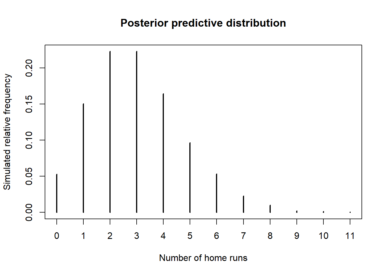
There is a posterior predictive probability of 95% of between 0 and 6 home runs in a game. Very roughly, about 95% of games have between 0 and 6 home runs.
quantile(y_sim, 0.95)## 95% ## 6Simulate a value of \(\theta\) from its Gamma(101, 34) posterior distribution, then given \(\theta\) simulate 32 values of \(y\) from a Poisson(\(\theta\)) distribution. Summarize each sample. Repeat many times to simulate many samples of size 32. Compare the observed sample with the simulated samples. Aside from the fact there the sample has no games with 0 home runs, the model seems reasonable.
df = read.csv("_data/citizens-bank-hr-2020.csv")
y = df$hr
n = length(y)

plot(table(y) / n, type = "h", xlim = c(0, 13), ylim = c(0, 0.4),
 xlab = "Number of home runs",
 ylab = "Observed/Simulated relative frequency",
 main = "Posterior predictive distribution")
axis(1, 0:13)

n_samples = 100


# simulate samples
for (r in 1:n_samples){

  # simulate theta from posterior distribution
  theta_sim = rgamma(1, 101, 34)

  # simulate values from Poisson(theta) distribution
  y_sim = rpois(n, theta_sim)

  # add plot of simulated sample to histogram
  par(new = T)
  plot(table(factor(y_sim, levels = 0:13)) / n, type = "o", xlim = c(0, 13), ylim = c(0, 0.4),
  xlab = "", ylab = "", xaxt='n', yaxt='n',
    col = rgb(135, 206, 235, max = 255, alpha = 25))
}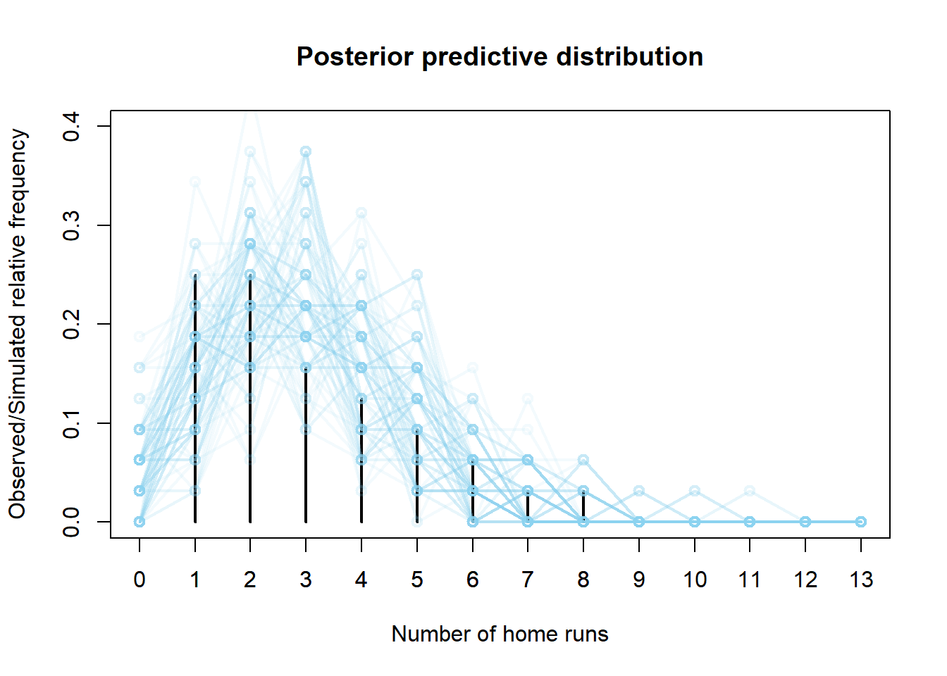
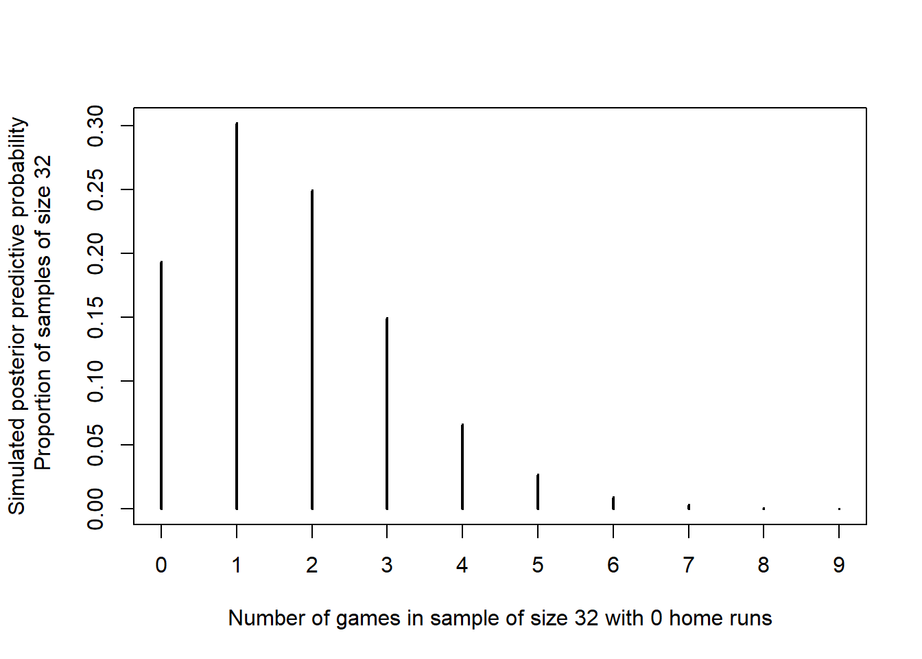
Continuing with the simulation from the previous part, now for each simulated sample we record the number of games with 0 home runs. Each “dot” in the plot below represents a sample of size 32 for which we measure the number of games in the sample with 0 home runs. While we see that it’s less likely to have 0 home runs in 32 games than not, it would not be too surprising to see 0 home runs in a sample of 32 games. Therefore, the fact that there are 0 home runs in the observed sample alone does not invalidate the model.
n_samples = 10000

zero_count = rep(NA, n_samples)

# simulate samples
for (r in 1:n_samples){

  # simulate theta from posterior distribution
  theta_sim = rgamma(1, 101, 34)

  # simulate values from Poisson(theta) distribution
  y_sim = rpois(n, theta_sim)
  zero_count[r] = sum(y_sim == 0)
}

par(mar = c(5, 5, 4, 2) + 0.1)
plot(table(zero_count) / n_samples, type = "h",
  xlab = "Number of games in sample of size 32 with 0 home runs",
  ylab = "Simulated posterior predictive probability\n Proportion of samples of size 32")