Chapter 5 Introduction to Estimation

A parameter is a number that describes the population, e.g., population mean, population proportion. The actual value of a parameter is almost always unknown.

A statistic is a number that describes the sample, e.g., sample mean, sample proportion. We can use observed sample statistics to estimate unknown population parameters.

Example 5.1 Most people are right-handed, and even the right eye is dominant for most people. In a 2003 study reported in Nature, a German bio-psychologist conjectured that this preference for the right side manifests itself in other ways as well. In particular, he investigated if people have a tendency to lean their heads to the right when kissing. The researcher observed kissing couples in public places and recorded whether the couple leaned their heads to the right or left. (We’ll assume this represents a randomly selected representative sample of kissing couples.)

The parameter of interest in this study is the population proportion of kissing couples who lean their heads to the right. Denote this unknown parameter \(\theta\); our goal is to estimate \(\theta\) based on sample data.

Let \(Y\) be the number of couples in a random sample of \(n\) kissing couples that lean to right. Suppose that in a sample of \(n=12\) couples \(y=8\) leaned to the right. We’ll start with a non-Bayesian analysis.

If you were to estimate \(\theta\) with a single number based on this sample data alone, intuitively what number would you pick?
For a general \(n\) and \(\theta\), what is the distribution of \(Y\)?
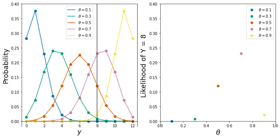
For the next few parts suppose \(n=12\). For a moment we’ll only consider these potential values for \(\theta\): \(0.1, 0.3, 0.5, 0.7, 0.9\). If \(\theta=0.1\) what is the distribution of \(Y\)? Compute and interpret the probability that \(Y=8\) if \(\theta = 0.1\).
If \(\theta=0.3\) what is the distribution of \(Y\)? Compute and interpret the probability that \(Y=8\) if \(\theta = 0.3\).
If \(\theta=0.5\) what is the distribution of \(Y\)? Compute and interpret the probability that \(Y=8\) if \(\theta = 0.5\).
If \(\theta=0.7\) what is the distribution of \(Y\)? Compute and interpret the probability that \(Y=8\) if \(\theta = 0.7\).
If \(\theta=0.9\) what is the distribution of \(Y\)? Compute and interpret the probability that \(Y=8\) if \(\theta = 0.9\).
Now remember that \(\theta\) is unknown. If you had to choose your estimate of \(\theta\) from the values \(0.1, 0.3, 0.5, 0.7, 0.9\), which one of these values would you choose based on of observing \(y=8\) couples leaning to the right in a sample of 12 kissing couples? Why?
Obviously our choice is not restricted to those five values of \(\theta\). Describe in principle the process you would follow to find the estimate of \(\theta\) based on of observing \(y=8\) couples leaning to the right in a sample of 12 kissing couples.
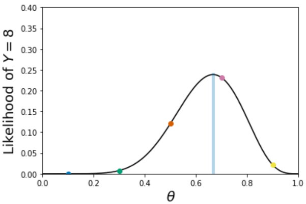
Let \(f(y|\theta)\) denote the probability of observing \(y\) couples leaning to the right in a sample of 12 kissing couples. Determine \(f(y=8|\theta)\) and sketch a graph of it. What is this a function of? What is an appropriate name for this function?
From the previous part, what seems like a reasonable estimate of \(\theta\) based solely on the data of observing \(y=8\) couples leaning to the right in a sample of 12 kissing couples?

\iffalse{} Solution. to Example 5.1

Show/hide solution

Seems reasonable to use the sample proportion 8/12 = 0.667.
\(Y\) has a Binomial(\(n\), \(\theta\)) distribution.
If \(\theta=0.1\) then \(Y\) has a Binomial(12, 0.1) distribution and \(P(Y = 8|\theta = 0.1) = \binom{12}{8}0.1^8(1-0.1)^{12-8}\approx 0.000\); dbinom(8, 12, 0.1).
If \(\theta=0.3\) then \(Y\) has a Binomial(12, 0.3) distribution and \(P(Y = 8|\theta = 0.3) = \binom{12}{8}0.3^8(1-0.3)^{12-8}\approx 0.008\); dbinom(8, 12, 0.3).
If \(\theta=0.5\) then \(Y\) has a Binomial(12, 0.5) distribution and \(P(Y = 8|\theta = 0.5) = \binom{12}{8}0.5^8(1-0.5)^{12-8}\approx 0.121\); dbinom(8, 12, 0.5).
If \(\theta=0.7\) then \(Y\) has a Binomial(12, 0.7) distribution and \(P(Y = 8|\theta = 0.7) = \binom{12}{8}0.7^8(1-0.7)^{12-8}\approx 0.231\); dbinom(8, 12, 0.7).
If \(\theta=0.9\) then \(Y\) has a Binomial(12, 0.9) distribution and \(P(Y = 8|\theta = 0.9) = \binom{12}{8}0.9^8(1-0.9)^{12-8}\approx 0.021\); dbinom(8, 12, 0.9).
Compare the above values, and see the plots below. The probability of observing \(y=8\) is greatest when \(\theta=0.7\), so in some sense the data seems most “consistent” with \(\theta=0.7\). The sample that we actually observed has the greatest likelihood of occurring when \(\theta = 0.7\) (among these choices for \(\theta\)). From a different perspective, if \(\theta=0.1\) then the likelihood of observing 8 successes in a sample of size 12 is very small. Therefore, since we actually did observed 8 successes in a sample of size 12, the data do not seem consistent with \(\theta=0.1\).
For each value of \(\theta\) between 0 and 1 compute the probability of observing \(y=8\), \(P(Y = 8|\theta)\), and find which value of \(\theta\) maximizes this probability.
\(f(y=8|\theta)=P(Y=8|\theta) = \binom{12}{8}\theta^8(1-\theta)^{12-8}\). This is a function of \(\theta\), with the data \(y=8\) fixed. Since this function computes the likelihood of observing the data (evidence) under different values of \(\theta\), “likelihood function” seems like an appropriate name. See the plots below.
The value which maximizes the likelihood of \(y=8\) is \(8/12\). So the maximum likelihood estimate of \(\theta\) is \(8/12\).

For given data \(y\), the likelihood function \(f(y|\theta)\) is the probability (or density for continuous data) of observing the sample data \(y\) viewed as a function of the parameter \(\theta\).
In the likelihood function, the observed value of the data \(y\) is treated as a fixed constant.
The value of a parameter that maximizes the likelihood function is called a maximum likelihood estimate (MLE).
The MLE depends on the data \(y\). For given data \(y\), the MLE is the value of \(\theta\) which gives the largest likelihood of having produced the observed data \(y\).
Maximum likelihood estimation is a common frequentist technique for estimating the value of a parameter based on data from a sample.

Example 5.2 We’ll now take a Bayesian approach to estimating \(\theta\) in Example 5.1. We treat the unknown parameter \(\theta\) as a random variable and wish to find its posterior distribution after observing \(y=8\) couples leaning to the right in a sample of 12 kissing couples.

We will start with a very simplified, unrealistic prior distribution that assumes only five possible, equally likely values for \(\theta\): 0.1, 0.3, 0.5, 0.7, 0.9.

Sketch a plot of the prior distribution and fill in the prior column of the Bayes table.
Now suppose that \(y=8\) couples in a sample of size \(n=12\) lean right. Sketch a plot of the likelihood function and fill in the likelihood column in the Bayes table.
Complete the Bayes table and sketch a plot of the posterior distribution. What does the posterior distribution say about \(\theta\)? How does it compare to the prior and the likelihood? If you had to estimate \(\theta\) with a single number based on this posterior distribution, what number might you pick?
Now consider a prior distribution which places probability 1/9, 2/9, 3/9, 2/9, 1/9 on the values 0.1, 0.3, 0.5, 0.7, 0.9, respectively. Redo the previous parts. How does the posterior distribution change?
Now consider a prior distribution which places probability 5/15, 4/15, 3/15, 2/15, 1/15 on the values 0.1, 0.3, 0.5, 0.7, 0.9, respectively. Redo the previous parts. How does the posterior distribution change?

\iffalse{} Solution. to Example 5.2

See plot below; the prior is “flat”.
The likelihood is computed as in Example 5.1. See the plots above.

See the Bayes table below. Since the prior is flat, the posterior is proportional to the likelihood. The values 0.7 and 0.5 account for the bulk of posterior plausibility, and 0.7 is about twice as plausible as 0.5. If we had to estimate \(\theta\) with a single number, we might pick 0.7 because that has the highest posterior probability.

theta = seq(0.1, 0.9, 0.2)

# prior

prior = rep(1, length(theta))
prior = prior / sum(prior)

# data
n = 12 # sample size
y = 8 # sample count of success

# likelihood, using binomial
likelihood = dbinom(y, n, theta) # function of theta

# posterior
product = likelihood * prior
posterior = product / sum(product)

# bayes table
bayes_table = data.frame(theta,
                     prior,
                     likelihood,
                     product,
                     posterior)

kable(bayes_table %>%
    adorn_totals("row"),
  digits = 4,
  align = 'r')

theta	prior	likelihood	product	posterior
0.1	0.2	0.0000	0.0000	0.0000
0.3	0.2	0.0078	0.0016	0.0205
0.5	0.2	0.1208	0.0242	0.3171
0.7	0.2	0.2311	0.0462	0.6065
0.9	0.2	0.0213	0.0043	0.0559
Total	1.0	0.3811	0.0762	1.0000

# plots
plot(theta-0.01, prior, type='h', xlim=c(0, 1), ylim=c(0, 1), col="skyblue", xlab='theta', ylab='')
par(new=T) 
plot(theta+0.01, likelihood/sum(likelihood), type='h', xlim=c(0, 1), ylim=c(0, 1), col="orange", xlab='', ylab='')
par(new=T)
plot(theta, posterior, type='h', xlim=c(0, 1), ylim=c(0, 1), col="seagreen", xlab='', ylab='')
legend("topleft", c("prior", "scaled likelihood", "posterior"), lty=1, col=c("skyblue", "orange", "seagreen"))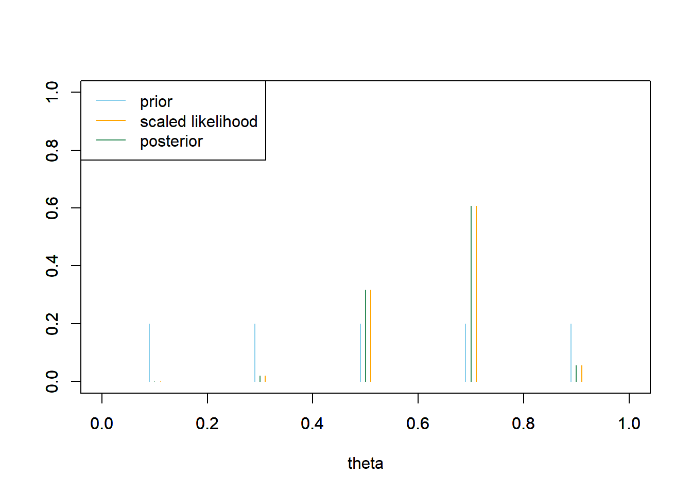

See table and plot below. Because the prior probability is now greater for 0.5 than for 0.7, the posterior probability of \(\theta=0.5\) is greater than in the previous part, and the posterior probability of \(\theta=0.7\) is less than in the previous part. The values 0.7 and 0.5 still account for the bulk of posterior plausibility, but now 0.7 is only about 1.3 times more plausible than 0.5. If we had to estimate \(\theta\) with a single number, we might pick 0.7 because that has the highest posterior probability.

theta	prior	likelihood	product	posterior
0.1	0.1111	0.0000	0.0000	0.0000
0.3	0.2222	0.0078	0.0017	0.0181
0.5	0.3333	0.1208	0.0403	0.4207
0.7	0.2222	0.2311	0.0514	0.5365
0.9	0.1111	0.0213	0.0024	0.0247
Total	1.0000	0.3811	0.0957	1.0000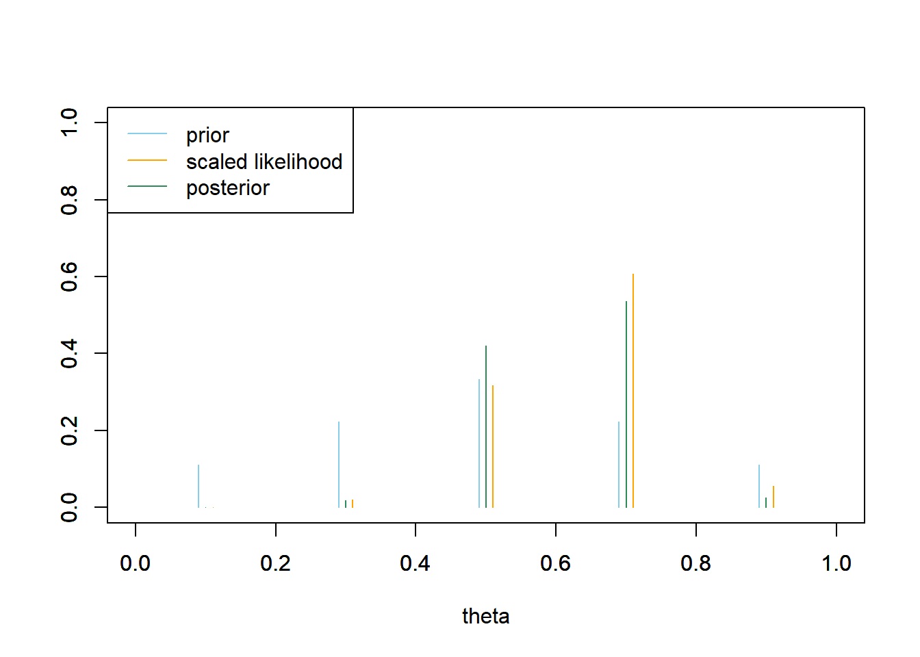

See the table and plot below. The prior probability is large for 0.1 and 0.3, but since the likelihood corresponding to these values is so small, the posterior probabilities are small. This posterior distribution is similar to the one from the previous part.

theta	prior	likelihood	product	posterior
0.1	0.3333	0.0000	0.0000	0.0000
0.3	0.2667	0.0078	0.0021	0.0356
0.5	0.2000	0.1208	0.0242	0.4132
0.7	0.1333	0.2311	0.0308	0.5269
0.9	0.0667	0.0213	0.0014	0.0243
Total	1.0000	0.3811	0.0585	1.0000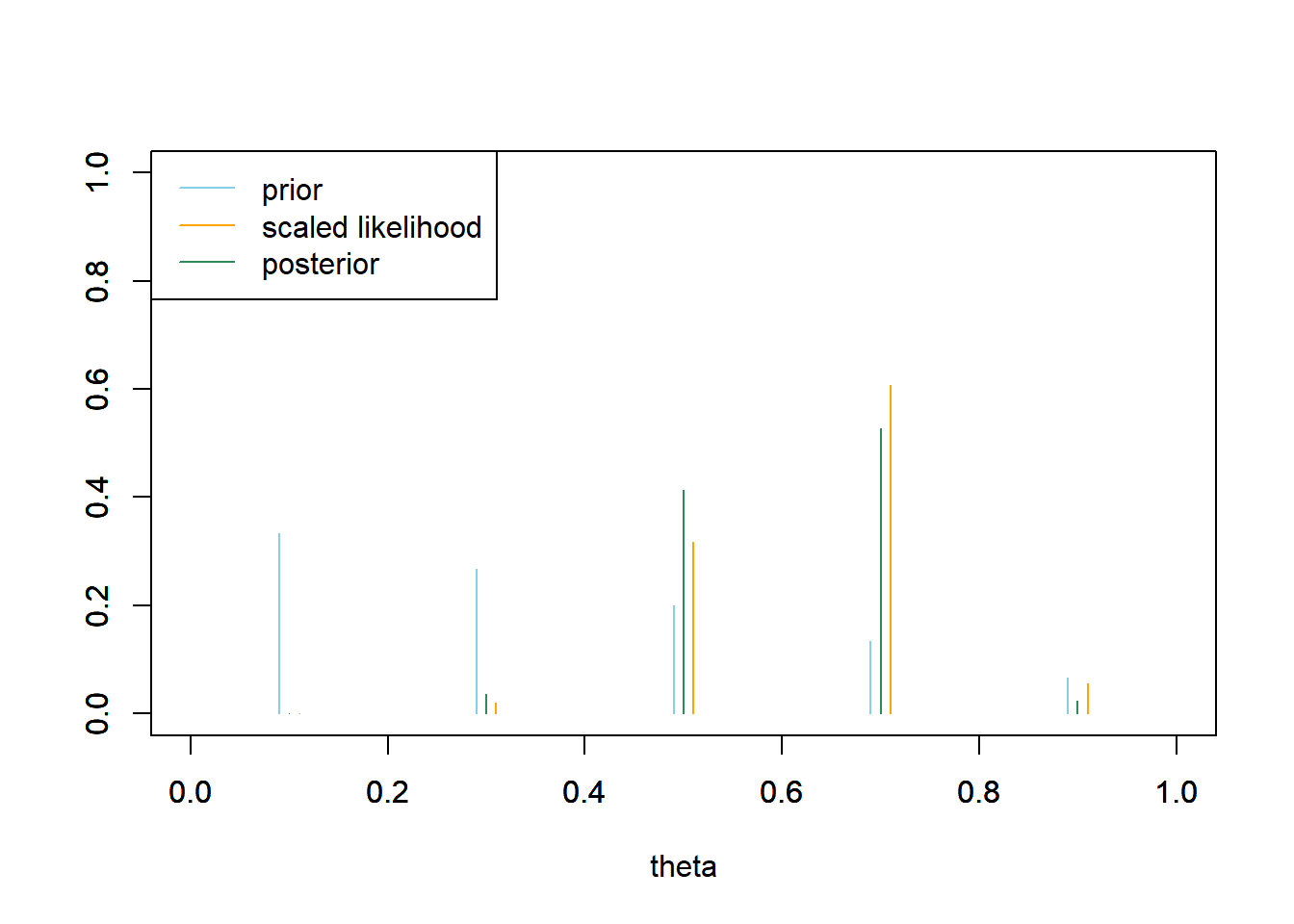

Bayesian estimation

Regards parameters as random variables with probability distributions
Assigns a subjective prior distribution to parameters
Conditions on the observed data
Applies Bayes’ rule to produce a posterior distribution for parameters \[ \text{posterior} \propto \text{likelihood} \times \text{prior} \]
Determines parameter estimates from the posterior distribution

In a Bayesian analysis, the posterior distribution contains all relevant information about parameters. That is, all Bayesian inference is based on the posterior distribution. The posterior distribution is a compromise between

prior “beliefs”, as represented by the prior distribution
data, as represented by the likelihood function

In contrast, a frequentist approach regards parameters as unknown but fixed (not random) quantities. Frequentist estimates are commonly determined by the likelihood function.

It is helpful to plot prior, likelihood, and posterior on the same plot. Since prior and likelihood are probability distributions, they are on the same scale. However, remember that the likelihood does not add up to anything in particular. To put the likelihood on the same scale as prior and posterior, it is helpful to rescale the likelihood so that it adds up to 1. Such a rescaling does not change the shape of the likelihood, it merely allows for easier comparison with prior and posterior.

Example 5.3 Continuing Example 5.2. While the previous exercise introduced the main ideas, it was unrealistic to consider only five possible values of \(\theta\).

What are the possible values of \(\theta\)? Does the parameter \(\theta\) take values on a continuous or discrete scale? (Careful: we’re talking about the parameter and not the data.)
Let’s assume that any multiple of 0.0001 is a possible value of \(\theta\): \(0, 0.0001, 0.0002, \ldots, 0.9999, 1\). Assume a discrete uniform prior distribution on these values. Suppose again that \(y=8\) couples in a sample of \(n=12\) kissing couples lean right. Use software to plot the prior distribution, the (scaled) likelihood function, and then find the posterior and plot it. Describe the posterior distribution. What does it say about \(\theta\)? If you had to estimate \(\theta\) with a single number based on this posterior distribution, what number might you pick?
Now assume a prior distribution which is proportional to \(1-2|\theta-0.5|\) for \(\theta = 0, 0.0001, 0.0002, \ldots, 0.9999, 1\). Use software to plot this prior; what does it say about \(\theta\)? Then suppose again that \(y=8\) couples in a sample of \(n=12\) kissing couples lean right. Use software to plot the prior distribution, the (scaled) likelihood function, and then find the posterior and plot it. What does the posterior distribution say about \(\theta\)? If you had to estimate \(\theta\) with a single number based on this posterior distribution, what number might you pick?
Now assume a prior distribution which is proportional to \(1-\theta\) for \(\theta = 0, 0.0001, 0.0002, \ldots, 0.9999, 1\). Use software to plot this prior; what does it say about \(\theta\)? Then suppose again that \(y=8\) couples in a sample of \(n=12\) kissing couples lean right. Use software to plot the prior distribution, the (scaled) likelihood function, and then find the posterior and plot it. What does the posterior distribution say about \(\theta\)? If you had to estimate \(\theta\) with a single number based on this posterior distribution, what number might you pick?
Compare the posterior distributions corresponding to the three different priors. How does each posterior distribution compare to the prior and the likelihood? Does the prior distribution influence the posterior distribution?

\iffalse{} Solution. to Example 5.3

The parameter \(\theta\) is a proportion, so it can possibly take any value in the continuous interval from 0 to 1.

See plot below. Since the prior is flat, the posterior is proportional to the likelihood. So the posterior distribution places highest posterior probability on values near the sample proportion 8/12. The interval of values from about 0.4 to 0.9 accounts for almost all of the posterior plausibility. If we had to estimate \(\theta\) with a single number, we might pick 8/12 = 0.667 because that has the highest posterior probability.

theta = seq(0, 1, 0.0001)

# prior
prior = rep(1, length(theta))
prior = prior / sum(prior)

# data
n = 12 # sample size
y = 8 # sample count of success

# likelihood, using binomial
likelihood = dbinom(y, n, theta) # function of theta


# plots
plot_posterior <- function(theta, prior, likelihood){

  # posterior
  product = likelihood * prior
  posterior = product / sum(product)

  ylim = c(0, max(c(prior, posterior, likelihood / sum(likelihood))))
  plot(theta, prior, type='l', xlim=c(0, 1), ylim=ylim, col="skyblue", xlab='theta', ylab='')
  par(new=T) 
  plot(theta, likelihood/sum(likelihood), type='l', xlim=c(0, 1), ylim=ylim, col="orange", xlab='', ylab='')
  par(new=T)
  plot(theta, posterior, type='l', xlim=c(0, 1), ylim=ylim, col="seagreen", xlab='', ylab='')
  legend("topleft", c("prior", "scaled likelihood", "posterior"), lty=1, col=c("skyblue", "orange", "seagreen"))
}

plot_posterior(theta, prior, likelihood)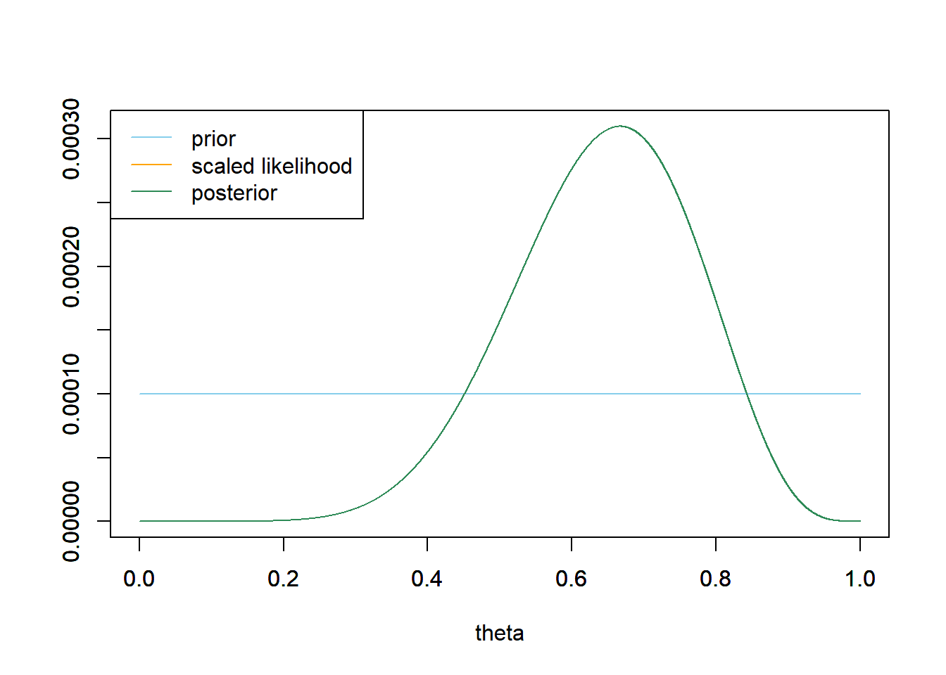

See plot below. The posterior is a compromise between the “triangular” prior which places highest prior probability near 0.5, and the likelihood. For this posterior, the posterior probability is greater near 0.5 than for the one in the previous part; the posterior here has been “shifted” towards 0.5 relative to the posterior from the previous part. If we had to estimate \(\theta\) with a single number, we might pick 0.615 because that has the highest posterior probability.
```
# prior
theta = seq(0, 1, 0.0001)
prior = 1 - 2 * abs(theta - 0.5)
prior = prior / sum(prior)

# data
n = 12 # sample size
y = 8 # sample count of success

# likelihood, using binomial
likelihood = dbinom(y, n, theta) # function of theta


# plots
plot_posterior(theta, prior, likelihood)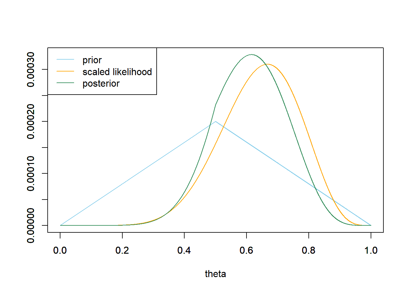
```
Again the posterior is a compromise between prior and likelihood. The prior probabilities are greatest for values of \(\theta\) near 0; however, the likelihood corresponding to these values is small, so the posterior probabilities are close to 0. As in the previous part, some of the posterior probability is shifted towards 0.5, as opposed to what happens with the uniform prior. The posterior here is fairly similar to the one from the previous part, and the maximum posterior probability still occurs around 0.61.
```
theta = seq(0, 1, 0.0001)

# prior
prior = 1 - theta
prior = prior / sum(prior)

# data
n = 12 # sample size
y = 8 # sample count of success

# likelihood, using binomial
likelihood = dbinom(y, n, theta) # function of theta

# plots
plot_posterior(theta, prior, likelihood)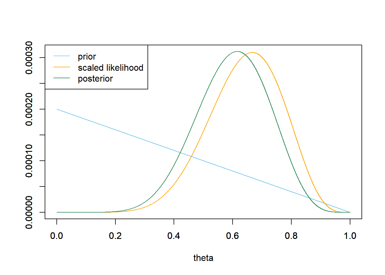
```
For the “flat” prior, the posterior is proportional to the likelihood. For the other priors, the posterior is a compromise between prior and likelihood. The prior does have some influence. We do see three somewhat different posterior distributions corresponding to these three prior distributions.

Even in situations where the data are discrete (e.g., binary success/failure data, count data), most statistical parameters take values on a continuous scale.
Thus in a Bayesian analysis, parameters are usually continuous random variables, and have continuous probability distributions, a.k.a., densities.
An alternative to dealing with continuous distributions is to use grid approximation: Treat the parameter as discrete, on a sufficiently fine grid of values, and use discrete distributions.

Example 5.4 Continuing Example 5.1. Now we’ll perform a Bayesian analysis on the actual study data in which 80 couples out of a sample of 124 leaned right. We’ll again use a grid approximation and assume that any multiple of 0.0001 between 0 and 1 is a possible value of \(\theta\): \(0, 0.0001, 0.0002, \ldots, 0.9999, 1\).

Before performing the Bayesian analysis, use software to plot the likelihood when \(y=80\) couples in a sample of \(n=124\) kissing couples lean right, and compute the maximum likelihood estimate of \(\theta\) based on this data. How does the likelihood for this sample compare to the likelihood based on the smaller sample (8/12) from previous exercises?
Now back to Bayesian analysis. Assume a discrete uniform prior distribution for \(\theta\). Suppose that \(y=80\) couples in a sample of \(n=124\) kissing couples lean right. Use software to plot the prior distribution, the likelihood function, and then find the posterior and plot it. Describe the posterior distribution. What does it say about \(\theta\)?
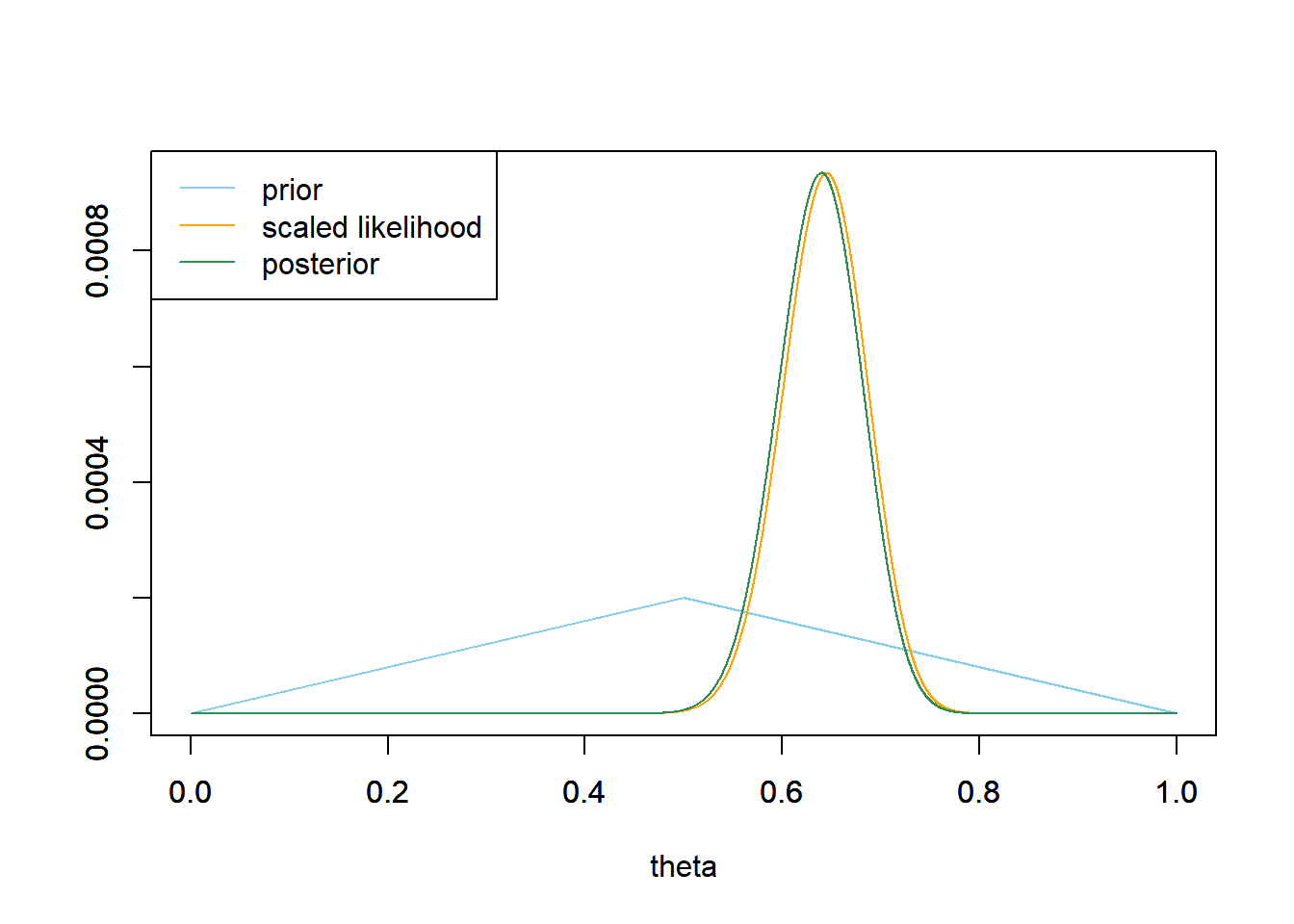
Now assume a prior distribution which is proportional to \(1-2|\theta-0.5|\) for \(\theta = 0, 0.0001, 0.0002, \ldots, 0.9999, 1\). Then suppose again that \(y=80\) couples in a sample of \(n=124\) kissing couples lean right. Use software to plot the prior distribution, the likelihood function, and then find the posterior and plot it. What does the posterior distribution say about \(\theta\)?
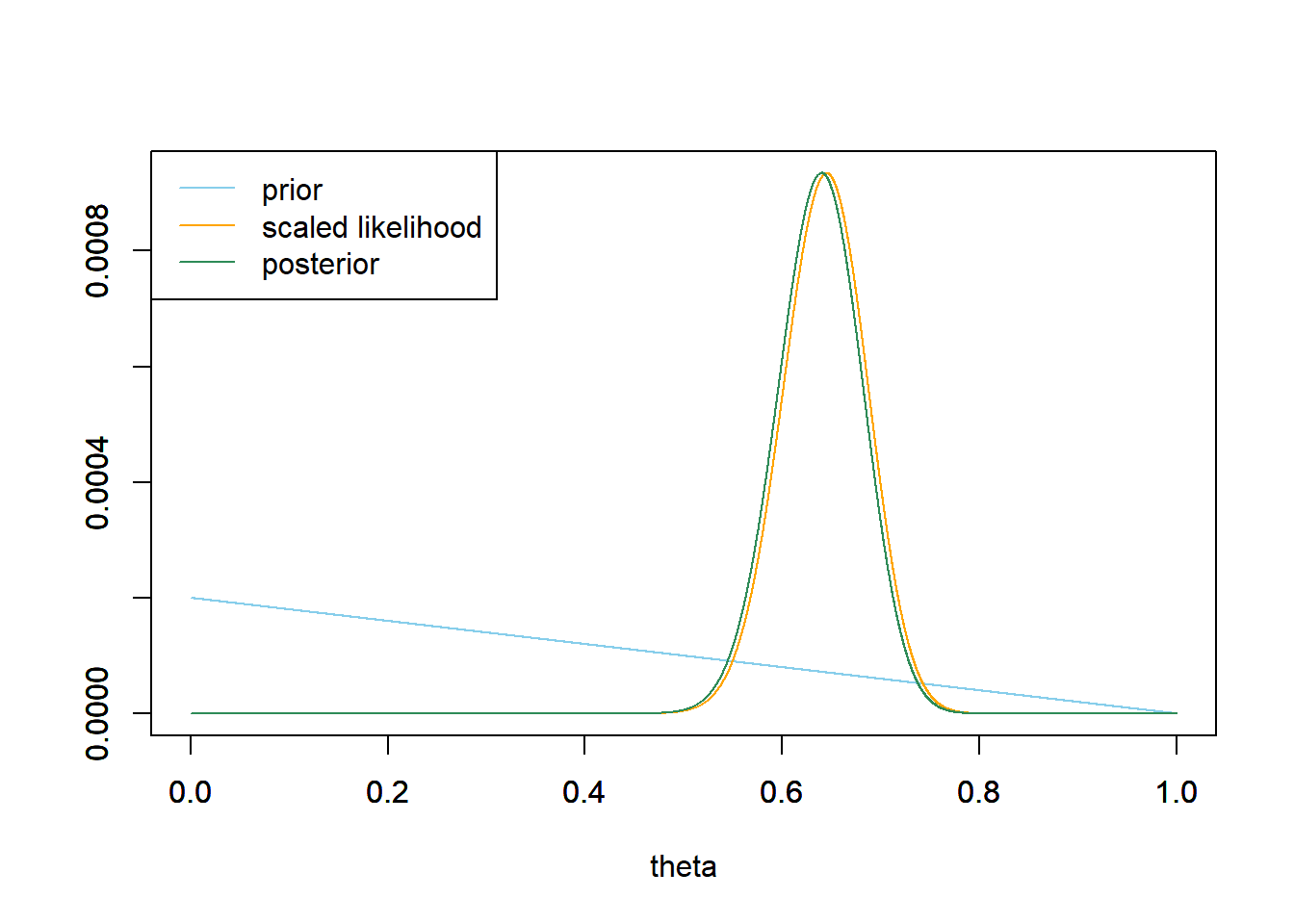
Now assume a prior distribution which is proportional to \(1-\theta\) for \(\theta = 0, 0.0001, 0.0002, \ldots, 0.9999, 1\). Then suppose again that \(y=80\) couples in a sample of \(n=124\) kissing couples lean right. Use software to plot the prior distribution, the likelihood function, and then find the posterior and plot it. What does the posterior distribution say about \(\theta\)?
Compare the posterior distributions corresponding to the three different priors. How does each posterior distribution compare to the prior and the likelihood? Comment on the influence that the prior distribution has. Does the Bayesian inference for these data appear to be highly sensitive to the choice of prior? How does this compare to the \(n=12\) situation?
If you had to produce a single number Bayesian estimate of \(\theta\) based on the sample data, what number might you pick?

\iffalse{} Solution. to Example 5.4

See plot below. The likelihood function is \(f(y=80|\theta) = \binom{124}{80}\theta^{80}(1-\theta)^{124-80}, 0 \le\theta\le1\), the likelihood of observing a value of \(y=80\) from a Binomial(124, \(\theta\)) distribution (dbinom(80, 124, theta)). The maximum likelihood estimate of \(\theta\) is the sample proportion \(80/124=0.645\). With the largest sample, the likelihood function is more “peaked” around its maximum.

See plot below. Since the prior is flat, the posterior is proportional to the likelihood. The posterior places almost all of its probability on \(\theta\) values between about 0.55 and 0.75, with the highest probability near the observed sample proportion of 0.645.

# prior
theta = seq(0, 1, 0.0001)
prior = rep(1, length(theta))
prior = prior / sum(prior)

# data
n = 124 # sample size
y = 80 # sample count of success

# likelihood, using binomial
likelihood = dbinom(y, n, theta) # function of theta

# plots
plot_posterior(theta, prior, likelihood)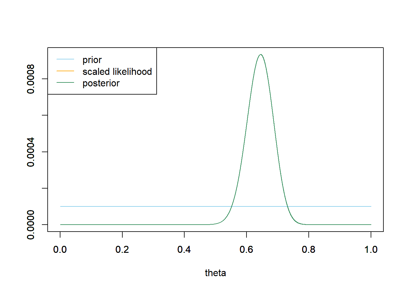

See the plot below. The posterior is very similar to the one from the previous part.
See the plot below. The posterior is very similar to the one from the previous part.
Even though the priors are different, the posterior distributions are all similar to each other and all similar to the shape of the likelihood. Comparing these priors it does not appear that the posterior is highly sensitive to choice of prior. The data carry more weight when \(n=124\) than it did when \(n=12\). In other words, the prior has less influence when the sample size is larger. When the sample size is larger, the likelihood is more “peaked” and so the likelihood, and hence posterior, is small outside a narrower range of values than when the sample size is small.
It seems that regardless of the prior, the posterior distribution is about the same, yielding the highest posterior probability around the sample proportion 0.645. So if we had to estimate \(\theta\) with a single number, we might just choose the sample proportion. In this case, we end up with the same numerical estimate of \(\theta\) in both the Bayesian and frequentist analysis. But the process and interpretation differs between the two approaches; we’ll discuss in more detail soon.