5.1 Point estimation

In a Bayesian analysis, the posterior distribution contains all relevant information about parameters after observing sample data. We often use certain summary characteristics of the posterior distribution to make inferences about parameters.

Example 5.5 Continuing the kissing study in Example 5.2 where \(\theta\) can only take values 0.1, 0.3, 0.5, 0.7, 0.9. Consider a prior distribution which places probability 5/15, 4/15, 3/15, 2/15, 1/15 on the values 0.1, 0.3, 0.5, 0.7, 0.9, respectively. Suppose we want a single number point estimate of \(\theta\). What are some reasonable choices?

Suppose we want a single number point estimate of \(\theta\) before observing sample data. Find the mode of the prior distribution of \(\theta\), a.k.a., the “prior mode”.
Find the median of the prior distribution of \(\theta\), a.k.a., the “prior median”.

Find the expected value of the prior distribution of \(\theta\), a.k.a., the “prior mean”.

Now suppose that \(y=8\) couples in a sample of size \(n=12\) lean right. Recall the Bayes table.

theta	prior	likelihood	product	posterior
0.1	0.3333	0.0000	0.0000	0.0000
0.3	0.2667	0.0078	0.0021	0.0356
0.5	0.2000	0.1208	0.0242	0.4132
0.7	0.1333	0.2311	0.0308	0.5269
0.9	0.0667	0.0213	0.0014	0.0243
Total	1.0000	0.3811	0.0585	1.0000

Find the mode of the posterior distribution of \(\theta\), a.k.a., the “posterior mode”.
Find the median of the posterior distribution of \(\theta\), a.k.a., the “posterior median”.
Find the expected value of the posterior distribution of \(\theta\), a.k.a., the “posterior mean”.
How have the posterior values changed from the respective prior values?

\iffalse{} Solution. to Example 5.5

Show/hide solution

The prior mode is 0.1, the value of \(\theta\) with the greatest prior probability.
The prior median is 0.3. Start with the smallest possible value of \(\theta\) and add up the prior probabilities until they go from below 0.5 to above 0.5. This happens when you add in the prior probability for \(\theta=0.3\).
The prior mean is 0.367. Remember that an expected value is a probability-weighted average value \[ 0.1(5/15) + 0.3(4/15) + 0.5(3/15) + 0.7(2/15) + 0.9(1/15) = 0.367. \]
The posterior mode is 0.7, the value of \(\theta\) with the greatest posterior probability.
The posterior median is 0.7. Start with the smallest possible value of \(\theta\) and add up the posterior probabilities until they go from below 0.5 to above 0.5. This happens when you add in the posterior probability for \(\theta=0.7\).
The posterior mean is 0.608. Now the posterior probabilities are used in the probability-weighted average value \[ 0.1(0.000) + 0.3(0.036) + 0.5(0.413) + 0.7(0.527) + 0.9(0.024) = 0.608. \]
The point estimates (mode, median, mean) shift from their prior values (0.1, 0.3, 0.367) towards the observed sample proportion of 8/12. However, the posterior distribution is not symmetric, and the posterior mean is less than the posterior median. In particular, note that the posterior mean (0.608) lies between the prior mean (0.367) and the sample proportion (0.667).

A point estimate of an unknown parameter is a single-number estimate of the parameter. Given a posterior distribution of a parameter \(\theta\), three possible Bayesian point estimates of \(\theta\) are:

the posterior mean
the posterior median
the posterior mode.

In particular, the posterior mean is the expected value of \(\theta\) according to the posterior distribution.

Recall that the expected value, a.k.a., mean, of a discrete random variable \(U\) is its probability-weighted average value \[ \text{E}(U) = \sum_u u\, P(U = u) \] In the calculation of a posterior mean, the parameter \(\theta\) plays the role of the random variable \(U\) and the posterior distribution provides the probability-weights.

In many situations, the posterior distribution will be roughly symmetric with a single peak, in which case posterior mean, median, and mode will all be about the same.

Reducing the posterior distribution to a single-number point estimate loses a lot of the information the posterior distribution provides. The entire posterior distribution quantifies the uncertainty about \(\theta\) after observing sample data. We will soon see how to more fully use the posterior distribution in making inference about \(\theta\).

Example 5.6 Continuing the kissing study in Example 5.3. Now assume a prior distribution which is proportional to \(1-\theta\) for \(\theta = 0, 0.0001, 0.0002, \ldots, 0.9999, 1\). Use software to answer the following.

Find the mode of the prior distribution of \(\theta\), a.k.a., the “prior mode”.
Find the median of the prior distribution of \(\theta\), a.k.a., the “prior median”.

Find the expected value of the prior distribution of \(\theta\), a.k.a., the “prior mean”.

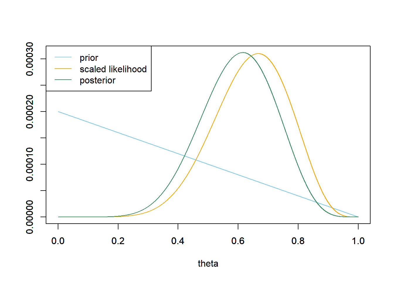
Now suppose that \(y=8\) couples in a sample of size \(n=12\) lean right. Recall the prior, likelihood, and posterior.

theta = seq(0, 1, 0.0001)

# prior
prior = 1 - theta # shape of prior
prior = prior / sum(prior) # scales so that prior sums to 1

# data
n = 12 # sample size
y = 8 # sample count of success

# likelihood, using binomial
likelihood = dbinom(y, n, theta) # function of theta

# posterior
product = likelihood * prior
posterior = product / sum(product)

Find the mode of the posterior distribution of \(\theta\), a.k.a., the “posterior mode”.
Find the median of the posterior distribution of \(\theta\), a.k.a., the “posterior median”.
Find the expected value of the posterior distribution of \(\theta\), a.k.a., the “posterior mean”.
How have the posterior values changed from the respective prior values?

\iffalse{} Solution. to Example 5.6

See the code below. The prior mode is 0.
See the code below. The prior median is 0.293.

See the code below. The prior mean is 0.333.

## prior

# prior mode
theta[which.max(prior)]

## [1] 0

# prior median
min(theta[which(cumsum(prior) >= 0.5)])

## [1] 0.2929

# prior mean
sum(theta * prior)

## [1] 0.3333

See the code below. The posterior mode is 0.615.
See the code below. The posterior median is 0.605.
See the code below. The posterior mean is 0.6.
Each of the posterior point estimates has shifted from its prior value towards the sample proportion of 0.667. But note that each of the posterior point estimates is in between the prior point estimate and the sample proportion.
```
## posterior

# posterior mode
theta[which.max(posterior)]
```
```
## [1] 0.6154
```
```
# posterior median
min(theta[which(cumsum(posterior) >= 0.5)])
```
```
## [1] 0.6046
```
```
# posterior mean
sum(theta * posterior)
```
```
## [1] 0.6
```

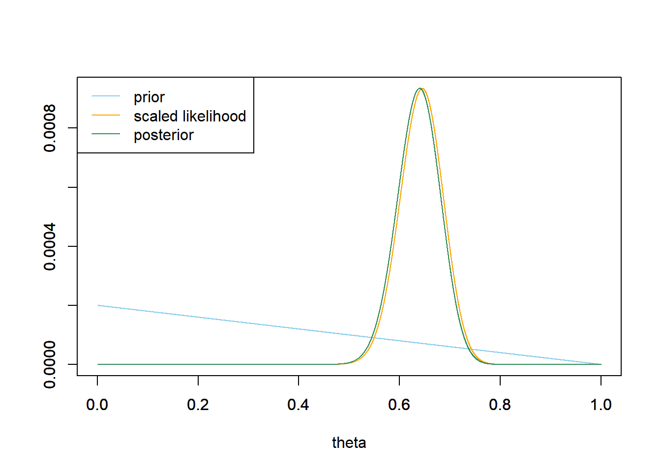
Example 5.7 Continuing Example 5.6, now suppose that \(y=80\) couples in a sample of size \(n=124\) lean right (the actual study data). Recall the prior, likelihood, and posterior.

# data
n = 124 # sample size
y = 80 # sample count of success

# likelihood, using binomial
likelihood = dbinom(y, n, theta) # function of theta

# posterior
product = likelihood * prior
posterior = product / sum(product)

Find the mode of the posterior distribution of \(\theta\), a.k.a., the “posterior mode”.
Find the median of the posterior distribution of \(\theta\), a.k.a., the “posterior median”.
Find the expected value of the posterior distribution of \(\theta\), a.k.a., the “posterior mean”.
How have the posterior values changed from the respective prior values? How does this compare to the smaller sample (8 out of 12)?

\iffalse{} Solution. to Example 5.7

See the code below. The posterior mode is 0.64.
See the code below. The posterior median is 0.639.
See the code below. The posterior mean is 0.638.
The posterior distribution is roughly symmetric, and posterior mean, median, and mode are about the same. Each of the posterior point estimates has shifted from its prior value towards the sample proportion of 0.645. The posterior point estimates are now closer to the sample proportion than they were with the smaller sample size. With the larger sample size, the data carry more weight.
```
## posterior

# posterior mode
theta[which.max(posterior)]
```
```
## [1] 0.64
```
```
# posterior median
min(theta[which(cumsum(posterior) >= 0.5)])
```
```
## [1] 0.6385
```
```
# posterior mean
sum(theta * posterior)
```
```
## [1] 0.6378
```