Chapter 20 Bayesian Analysis of Simple Linear Regression

Regression is one of the most widely used statistical techniques for modeling relationships between variables. We will now consider a Bayesian treatment of simple linear regression. We’ll use the following example throughout.

Percent body fat (PBF, total mass of fat divided by total body mass) is an indicator of physical fitness level, but it is difficult to measure accurately. Body mass index (BMI), which is easily computed based on height and weight (\(\text{BMI} = \frac{\text{weight in kg}}{\text{(height in m)}^2}\)), is another commonly used measure⁴². What is the relationship between BMI and percent body fat? How can we use a person’s BMI to estimate their percent body fat?

Example 20.1 We’ll consider a Bayesian simple linear regression model for predicting percent body fat from BMI.

What are the assumptions of the simple linear regression model? (There are many different regression models. We’re referring to the one that is usually the first one you see in introductory statistics. Sometimes the assumptions are introduced with the acronym “LINE”.)
What are the parameters in the model? That is, what do we need to put a prior distribution on (in order to eventually get a posterior distribution given sample data)?
Suggest a prior distribution.
Simulate the prior predictive distribution of percent body fat for a range of BMI values. Does the distribution seem reasonable?
Experiment with different priors until you find one that produces a reasonable prior predictive distribution.

\iffalse{} Solution. to Example 20.1

The regression model assumes that mean percent body fat is a linear function of BMI. Among men with the same BMI, values of percent body fat are Normally distributed with a mean that depends on BMI and some (conditional) standard deviation. See below for the general assumptions.
The parameters are the slope \(\beta_1\), the intercept \(\beta_0\), and the (conditional) standard deviation \(\sigma\). The parameters \(\beta_0\) and \(\beta_1\) are related to the conditional mean of \(Y\) given \(x\), and the parameter \(\sigma\) is the conditional SD of \(Y\) given \(x\).
We’ll assume a prior under which \(\beta_0\), \(\beta_1\), and \(\sigma\) are independent. A quick Google search reveals that for men percent body fat ranges from about 6% to 30%, and BMI ranges from about 15 to 35 kg/m². If we assume percent body fat varies by about 5 percent among men of the same BMI, we can choose a prior for \(\sigma\) that has a mean of 5, say Exponential(1/5). We expect a positive association between percent body fat and BMI, so we want a prior for \(\beta_1\) that places most of its credibility on positive values. Disregarding measurement units, the two variables take values on similar numerical scales. For the slope \(\beta_1\), we might assume a Normal prior with a mean of 1 and a standard deviation of 0.5 (to keep most of the credibility on positive values). The intercept \(\beta_0\), in principle, represents the percent body fat for a man with a BMI of 0, so we might assume a Normal prior with a mean of 0 and a standard deviation of 1 (to put most of the prior credibility near 0).
Given a value of BMI \(x\), first simulate \(\beta_0, \beta_1\), and \(\sigma\) from the joint prior distribution, then simulate a value of percent body fat \(y\) from a Normal distribution with mean \(\beta_0 + \beta_1x\) and standard deviation \(\sigma\). For example, for simulated \(\beta_0 = 0.1\), \(\beta_1 = 0.8\), and \(\sigma = 4.2\) and a given \(x = 20\), we would simulate \(y\) from a Normal distribution with mean \(0.1 + 0.8(20)\) and standard deviation 4.2.

The code below simulates a sample of 1000 pairs.
```
Nrep = 1000

x = rnorm(Nrep, 25, 5) # just some possible values of BMI

beta0 = rnorm(Nrep, 0, 1)
beta1 = rnorm(Nrep, 1, 0.5)
sigma = rexp(Nrep, 1 / 5)

y = rnorm(Nrep, beta0 + beta1 * x, sigma)

plot(x, y, xlab = "BMI (kg/m^2)", ylab = "Percent body fat (%)")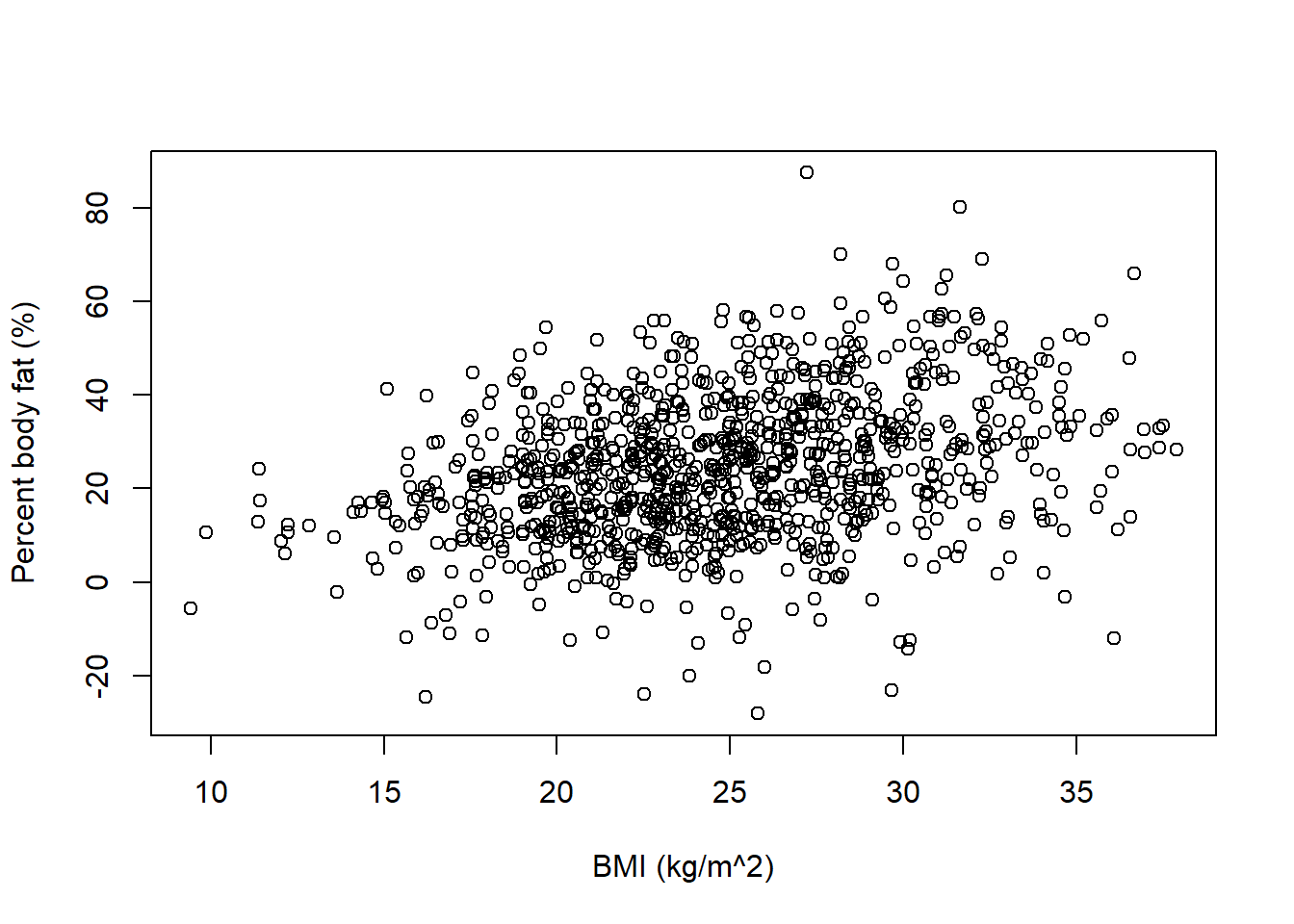
```
The code below simulates what some possible regression lines might look like. Remember, the regression line represents the mean percent body fat for any given value of BMI.
```
nlines = 100

plot(x, y, xlab = "BMI (kg/m^2)", ylab = "Percent body fat (%)", type = "n",
 xlim = c(15, 35),
 ylim = c(0, 30))


for (l in 1:nlines){
  abline(beta0[l], beta1[l], col = "skyblue", lwd = 1)
}
```
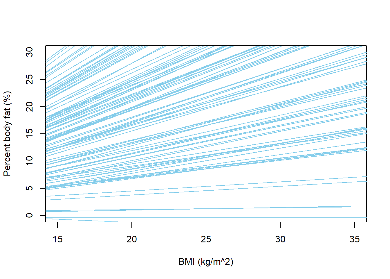
We can tell from these plots that there are problems with the model. The model predicts many negative values of percent body fat. The possible regression lines are all over the place, indicating that for almost any given BMI, the mean percent body fat can be anywhere from 0 to 30 (or more) percent. We also see a few negative slopes, which doesn’t seem realistic. Therefore, we should revise our assumptions so that our prior predictive distribution produces more reasonable values of percent body fat.
The previous part illustrates that when there are multiple parameters it can be difficult to interpret the prior distribution of any particular parameter in isolation. For example, the intercept in theory should be 0; however, a BMI of 0 is unreasonable and would never appear in the data. The intercept needs to work together with the slope so that men with average BMI have average percent body fat.

The code below reflects one choice of prior, arrived at after some tuning. There are many others, and no one prior will be perfect. What’s important is that the prior distribution works together with the model for the data to produce reasonable values of the variables.

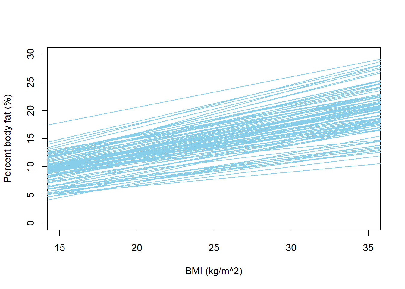
We see that with the prior below, fewer extreme values of percent body fat are predicted, most notably far fewer negative values than before. The possible regression lines do a better job of spanning the scale of percent body fat variable. For any given BMI, the prior range of plausible values for mean percent body fat is much narrower than before.

Nrep = 1000

beta0 = rnorm(Nrep, 2, 2)
beta1 = rnorm(Nrep, 0.5, 0.1)
sigma = rexp(Nrep, 1 / 1.5)

y = rnorm(Nrep, beta0 + beta1 * x, sigma)

plot(x, y, xlab = "BMI (kg/m^2)", ylab = "Percent body fat (%)")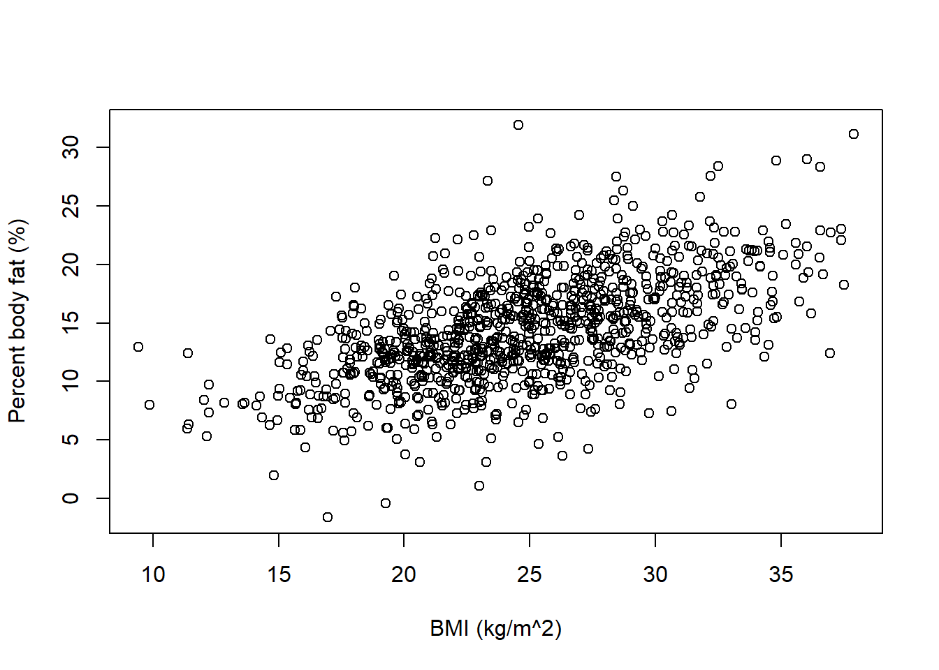

nlines = 100

plot(x, y, xlab = "BMI (kg/m^2)", ylab = "Percent body fat (%)", type = "n",
     xlim = c(15, 35),
     ylim = c(0, 30))


for (l in 1:nlines){
  abline(beta0[l], beta1[l], col = "skyblue", lwd = 1)
}

Consider data on a response variable \(Y\) and an explanatory variable \(x\). A simple linear regression model of \(Y\) on \(x\) assumes

Linearity: the conditional mean of \(Y\) is in \(x\); for some \(\beta_0, \beta_1\) and every \(x\) \[ E(Y|X=x) = \beta_0 + \beta_1 x \]
Independence: \(Y_1,\ldots, Y_n\) are independent.
Normality: for each \(x\), the conditional distribution of \(Y\) given \(X=x\) is Normal
Equal variance: the conditional variance of \(Y\) does not depend on \(x\); for each \(x\) \[ Var(Y|X=x) = \sigma^2 \]

The regression model above is conditional. That is, we make assumptions about and perform inference for the conditional distribution of the response variable \(Y\) given values of the explanatory variable \(x\). Therefore, even when we technically have a sample of pairs \((X_i,Y_i)\) from a bivariate distribution, we will always condition on the values of \(X\) and treat them as non-random.

Linearity is an assumption: we assume there is some “true” population regression line \(\beta_0 + \beta_1 x\) which specifies the conditional mean of the response variable for each value of the explanatory variable.

The above set of assumptions can be stated more compactly as \[ Y_i \sim N\left( \beta_0 + \beta_1 x_i, \sigma^2\right), \text{ and } Y_1, \ldots, Y_n \text{ are independent} \] Equivalently, \[ Y_i = \beta_0 + \beta_1 x_i + \varepsilon_i, \text{ where } \varepsilon_i, \ldots, \varepsilon_n \text{ are i.i.d. } N(0,\sigma^2). \]

The parameters of the above model are \(\beta_0\), \(\beta_1\), and \(\sigma^2\). Note that \(\sigma_Y^2\) denotes the variance of the response variable \(Y\) with respect to its overall mean, while \(\sigma^2\) denotes the variance of values of the response variable about the true regression line. Thus, \(\sigma^2 = (1-\rho^2)\sigma^2_Y\), where \(\rho\) is the population correlation between the explanatory and response variables.

The assumptions of the linear regression model can be relaxed in a number of ways, some of which we’ll mention briefly at the end of the section.

In models with multiple parameters, it can be difficult to interpret the prior or posterior distribution of any single parameter in isolation. Therefore, it becomes even more important to check predictive distributions for reasonableness. Do the prior and likelihood fit together to produce a reasonable distribution of values of the response variable? At the very least, the predicted values should lie in a reasonable range of the measurement unit scale of the variable. But remember: the prior distribution is just a starting point; it doesn’t have to be perfect (it never will be), just reasonable. Rather than fussing over the prior, we should focus our attention on the posterior distribution given sample data.

The following summarizes data on a nationally representative sample of 2157 U.S. males from the National Health and Nutrition Examination Survey (NHANES).

myData = read.csv("_data/nhanes_males.csv")
y = myData$PBF
x = myData$BMI
n = length(y)

hist(y, xlab = "Percent body fat (%)", main = paste("Mean=", mean(y), ", SD=", sd(y)))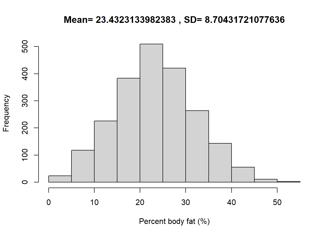

hist(x, xlab = "BMI (kg/m^2)", main = paste("Mean=",mean(x), ", SD=", sd(x)))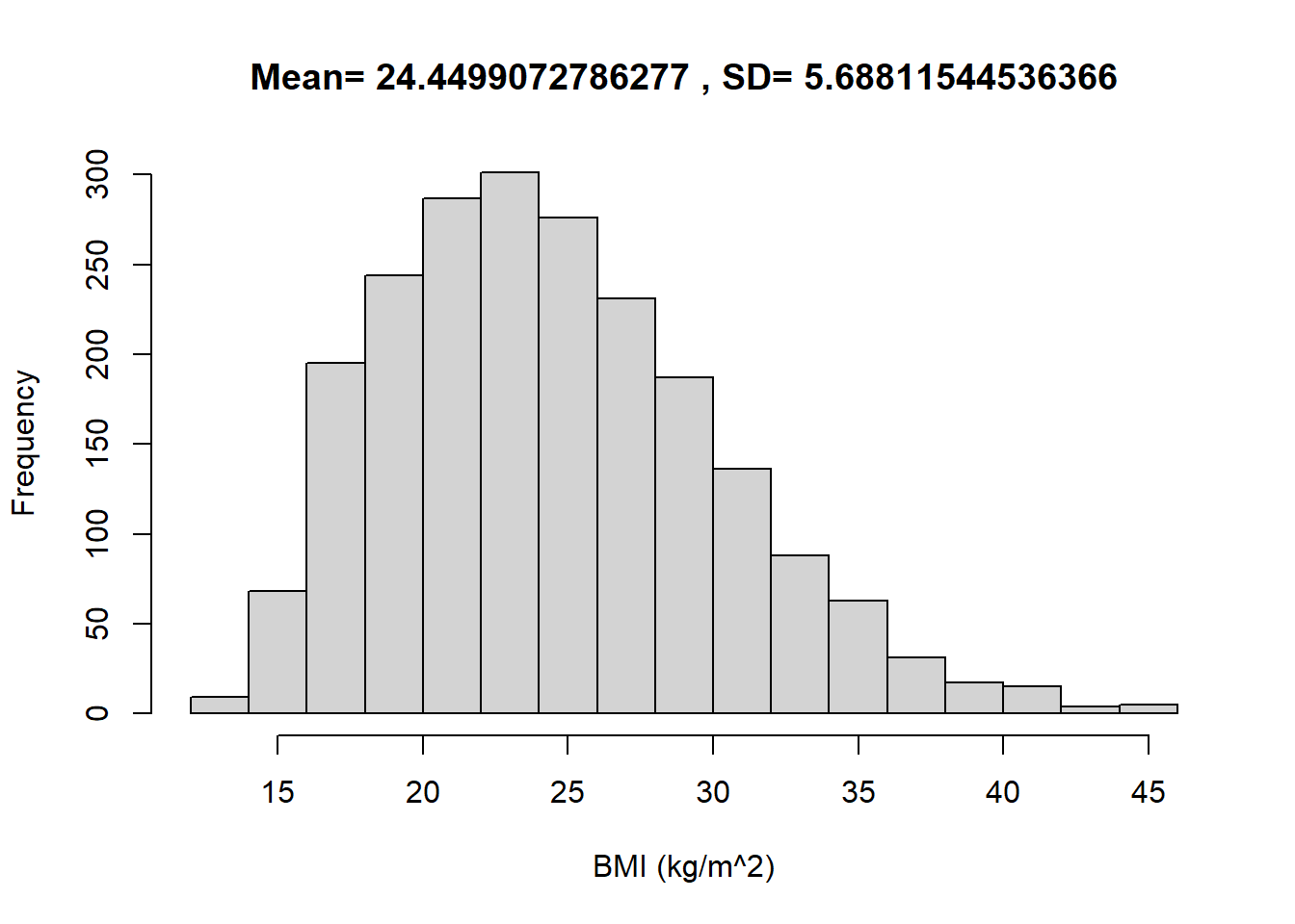

plot(x, y, xlab = "BMI (kg/m^2)", ylab = "Percent body fat (%)", main = paste("Correlation=", cor(x, y)))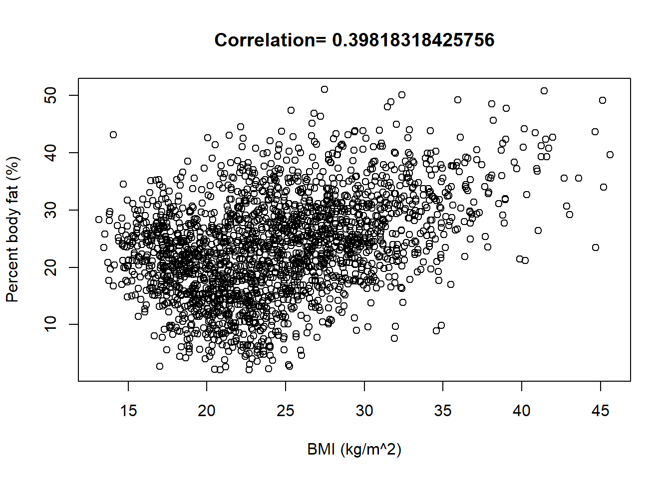

Example 20.2 Continuing the previous example, now we’ll use JAGS to find the posterior distribution given the sample data.

For the prior assume

\(\beta_0\), \(\beta_1\), and \(\sigma\) are independent
\(\beta_0\) has a Normal(2, 2) distribution
\(\beta_1\) has a Normal(0.5, 1) distribution
\(\sigma\) has an Exponential distribution with rate 1/1.5

Suppose there are just two observations of (BMI, PBF): (15, 20) and (40, 30). How would you compute the likelihood?
Use JAGS to fit the Bayesian model to the data. Inspect diagnostic plots; do you notice any problems?

\iffalse{} Solution. to Example 20.2

The assumptions of the regression model define the likelihood. Given a BMI of 15, PBFs follow a Normal distribution with mean \(\beta_0+15\beta_1\), so we would evaluate the likelihood of a PBF of 20 using a \(N(\beta_0+15\beta_1, \sigma)\) distribution: dnorm(20, beta0 + 15 * beta1, sigma). Similarly the likelihood for the observation (40, 30) is dnorm(40, beta0 + 30 * beta1, sigma). Since the regression model assumes independence between the response values, the likelihood for the sample would be, as a function of \((\beta_0, \beta_1, \sigma)\), proportional to \[ \propto \left[\frac{1}{\sigma}\exp\left(-\frac{1}{2}\left(\frac{20-(\beta_0+15\beta_1)}{\sigma}\right)^2\right)\right]\left[\frac{1}{\sigma}\exp\left(-\frac{1}{2}\left(\frac{40-(\beta_0+30\beta_1)}{\sigma}\right)^2\right)\right] \]
The JAGS code is below. For observation i, the likelihood of y[i] is determined using the Normal distribution with mean \(\beta_0 + \beta_1 x_i\) and SD \(\sigma\): y[i] ~ dnorm(beta[1] + beta[2] * x[i], 1 / sigma ^ 2). (Remember: JAGS uses precision for dnorm, and JAGS indices start at 1.) Diagnostics for \(\sigma\) seem fine. However, we notice that \(\beta_0\) and \(\beta_1\) have pretty low effective sample sizes and autocorrelations that decay to 0 fairly slowly. We’ll discuss further below.

library(rjags)

model_string <- "model{

  # Likelihood
  for(i in 1:n){
    y[i] ~ dnorm(mu[i], 1 / sigma ^ 2)
    mu[i] <- beta[1] + beta[2] * x[i]
  }

  # Prior for beta
  beta[1] ~ dnorm(2, 1 / 2 ^ 2)
  beta[2] ~ dnorm(0.5, 1 / 0.1 ^ 2)

  # Prior for sigma
  sigma ~ dexp(1 / 1.5)

}"

model <- jags.model(textConnection(model_string), 
                    data=list(n = n, y = y, x = x),
                    n.chains = 5)

## Compiling model graph
##    Resolving undeclared variables
##    Allocating nodes
## Graph information:
##    Observed stochastic nodes: 2157
##    Unobserved stochastic nodes: 3
##    Total graph size: 7016
## 
## Initializing model

update(model, 1000, progress.bar = "none"); # Burnin for 1000 samples

posterior_sample <- coda.samples(model, 
                                 variable.names = c("beta", "sigma"), 
                                 n.iter = 10000, progress.bar = "none")

summary(posterior_sample)

## 
## Iterations = 2001:12000
## Thinning interval = 1 
## Number of chains = 5 
## Sample size per chain = 10000 
## 
## 1. Empirical mean and standard deviation for each variable,
##    plus standard error of the mean:
## 
##          Mean     SD Naive SE Time-series SE
## beta[1] 7.969 0.6892 0.003082       0.017320
## beta[2] 0.631 0.0275 0.000123       0.000692
## sigma   7.983 0.1221 0.000546       0.000685
## 
## 2. Quantiles for each variable:
## 
##          2.5%   25%   50%   75% 97.5%
## beta[1] 6.628 7.500 7.966 8.433 9.323
## beta[2] 0.577 0.612 0.631 0.649 0.684
## sigma   7.749 7.899 7.981 8.064 8.226

plot(posterior_sample)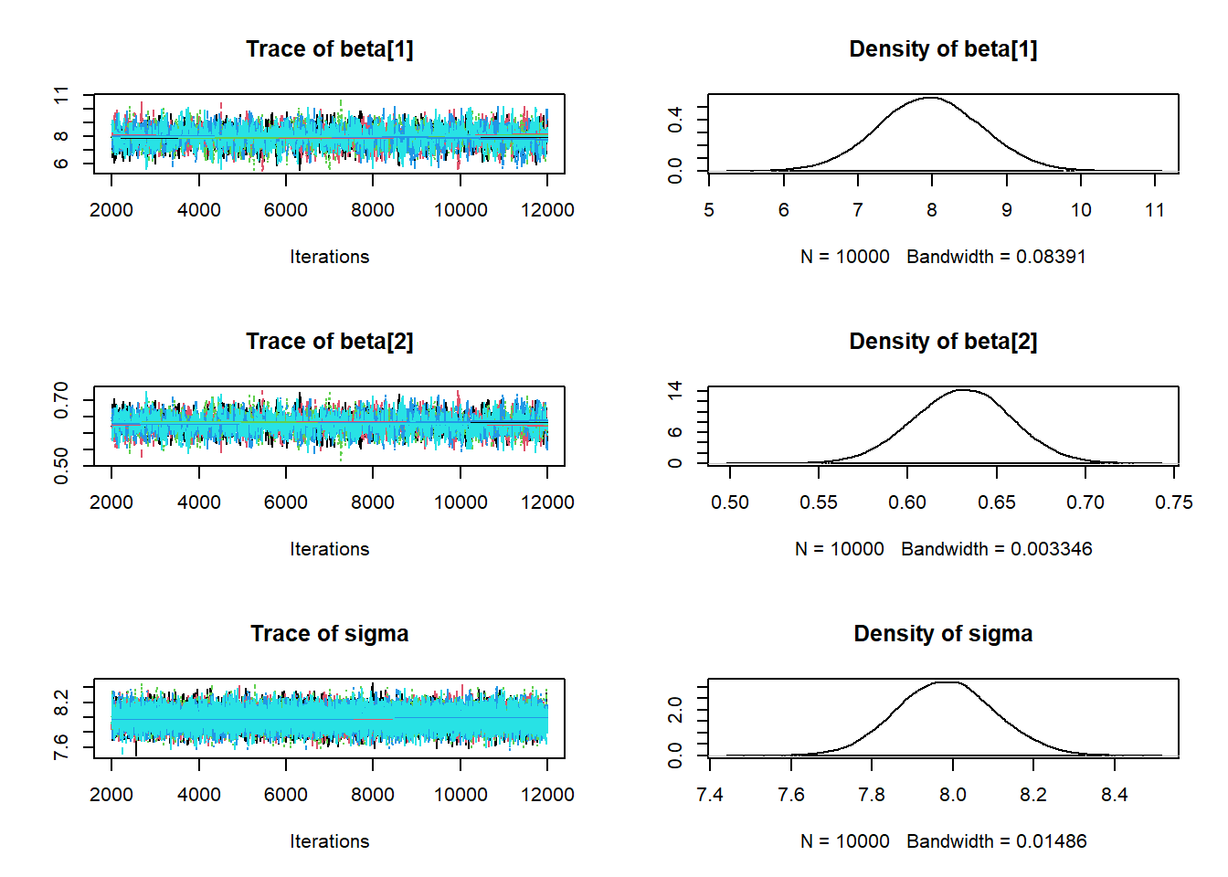

params = as.matrix(posterior_sample)
beta0 = params[, 1]
beta1 = params[, 2]
sigma = params[, 3]

mcmc_acf(posterior_sample)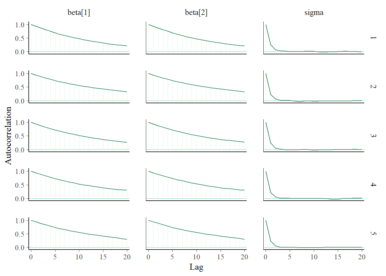

mcmc_trace(posterior_sample)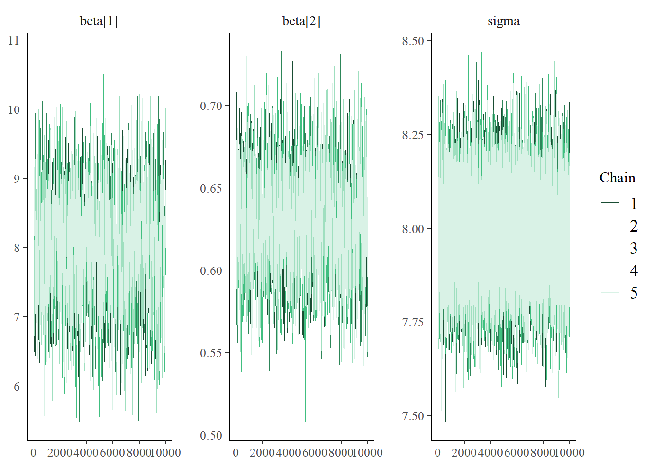

plotPost(beta0)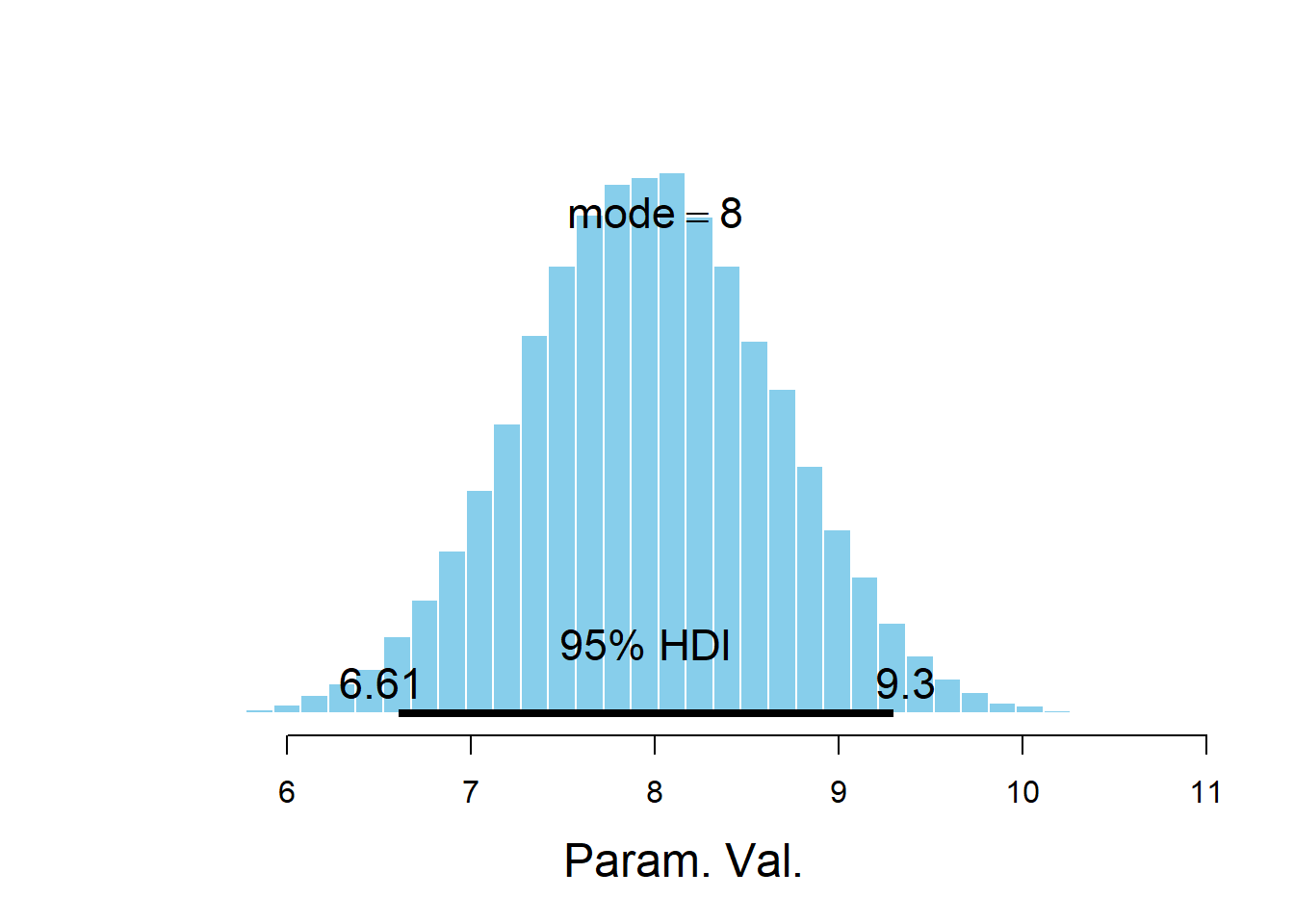

##              ESS  mean median  mode hdiMass hdiLow hdiHigh compVal pGtCompVal
## Param. Val. 1600 7.969  7.966 8.002    0.95  6.605   9.297      NA         NA
##             ROPElow ROPEhigh pLtROPE pInROPE pGtROPE
## Param. Val.      NA       NA      NA      NA      NA

plotPost(beta1)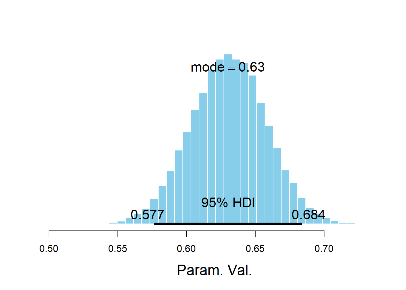

##              ESS   mean median   mode hdiMass hdiLow hdiHigh compVal pGtCompVal
## Param. Val. 1583 0.6307  0.631 0.6301    0.95 0.5767   0.684      NA         NA
##             ROPElow ROPEhigh pLtROPE pInROPE pGtROPE
## Param. Val.      NA       NA      NA      NA      NA

plotPost(sigma)

##               ESS  mean median  mode hdiMass hdiLow hdiHigh compVal pGtCompVal
## Param. Val. 30962 7.983  7.981 8.003    0.95  7.752   8.228      NA         NA
##             ROPElow ROPEhigh pLtROPE pInROPE pGtROPE
## Param. Val.      NA       NA      NA      NA      NA

We can tell from the diagnostic plots above that there is something amiss with the MCMC algorithm that JAGS is running. As we mentioned in Chapter 17 there are many different MCMC algorithms. We mainly studied the Metropolis algorithm, but this is just one of many MCMC algorithms. JAGS uses a number of different algorithms, but it is primarily based on Gibbs sampling. (JAGS stands for “Just Another Gibbs Sampler”.) It turns out that Gibbs sampling does not work very well for sampling from the posterior distribution in the previous situation.

Here is a brief description for how Gibbs sampling works to simulate \((\beta_0, \beta_1)\) pairs from their joint posterior distribution.

Start with some initial \((\beta_0, \beta_1)\) pair, say (0, 0).
A new \((\beta_0, \beta_1)\) pair is generated in two steps
- Given \(\beta_0\), generate a value of \(\beta_1\) from the conditional distribution of \(\beta_1\) given \(\beta_0\). (For example, if \((\beta_0, \beta_1)\) has a Bivariate Normal distribution, then conditional on \(\beta_0\), \(\beta_1\) has a Normal distribution with a mean that depends on \(\beta_0\).)
- Given \(\beta_1\), generate a value of \(\beta_0\) from the conditional distribution of \(\beta_0\) given \(\beta_1\).

Remember that MCMC algorithms generally involve two stages: proposal and acceptance/rejection. In Gibbs sampling the proposals are made according to conditional distributions and they are always accepted.

Let’s look at the simulated posterior joint distribution of \(\beta_0\) and \(\beta_1\) to see why Gibbs sampling is inefficient.

mcmc_scatter(posterior_sample,
             pars = c("beta[1]", "beta[2]"),
             alpha = 0.25)

In the scatterplot, we see a strong posterior correlation between \(\beta_0\) and \(\beta_1\). The conditional variance of \(\beta_1\) given \(\beta_0\) is fairly small. Therefore, starting from a \((\beta_0, \beta_1)\) pair, the next value of \(\beta_1\) will be fairly close to the current value of \(\beta_1\); similarly for \(\beta_0\). Essentially, the strong correlation puts up “walls” that the Gibbs sampler keeps slamming into, making it hard to go anywhere. So the Gibbs sampling Markov chain which generates values of \((\beta_0, \beta_1)\) takes only small steps, which leads to strong autocorrelation and small effective sample sizes.

The problem that we’re seeing is due to the Gibbs sampling algorithm, not with the model. The posterior distribution is what it is — there is nothing wrong with it — Gibbs sampling just doesn’t sample from it very efficiently. We could solve the problem by using another MCMC algorithm which makes more efficient proposals, such as Hamiltonian Monte Carlo in Stan. However, we can also make a small change to the model that helps Gibbs sampling run more efficiently.

Example 20.3 We’ll now consider a model with \(x\) (BMI) replaced with \(x-\bar{x}\).

Before fitting the model, let’s think about why this change might help. We saw a strong negative correlation between \(\beta_0\) and \(\beta_1\) above. Why should this negative correlation not be surprising? (Think about the least squares estimates of \(\beta_0\) and \(\beta_1\).)
How does replacing \(x\) with \(x-\bar{x}\) help with the issue in the previous part?
Use JAGS to fit the model. Compare the diagnostic summaries with those from the previous example. Does Gibbs sampling seem to work more efficiently when the explanatory variable is centered?

\iffalse{} Solution. to Example 20.3

The least squares regression line always passes through the point of the means \((\bar{x}, \bar{y})\). Since \(\bar{x}>0\), if the slope increases then the intercept must decrease. Similar ideas apply to the distribution of \(\beta_0\) and \(\beta_1\).
The centered variable \(x-\bar{x}\) has mean 0, and the least squares estimate of the intercept \(\beta_0\) is \(\bar{y}\), regardless of the slope. In this case, we expect the posterior distribution of \(\beta_0\) to be centered close to \(\bar{y}\), regardless of the slope \(\beta_0\). That is, we expect the posterior correlation between \(\beta_0\) and \(\beta_1\) to be close to 0. The problem Gibbs sampling encountered was due to the strong correlation. If we eliminate this correlation, Gibbs sampling should run more efficiently.
See below for the JAGS code. We replaced x with xc = x - mean(x), but otherwise the code is similar to before. The diagnostics for \(\beta_0\) and \(\beta_1\) look much better, with autocorrelations decaying quickly to 0 and large effective sample sizes.

xc = x - mean(x)

model_string <- "model{

  # Likelihood
  for(i in 1:n){
    y[i] ~ dnorm(mu[i], 1 / sigma ^ 2)
    mu[i] <- beta[1] + beta[2] * xc[i]
  }

  # Prior for beta
  beta[1] ~ dnorm(2, 1 / 2 ^ 2)
  beta[2] ~ dnorm(0.5, 1 / 0.1 ^ 2)

  # Prior for sigma
  sigma ~ dexp(1 / 1.5)

}"

model <- jags.model(textConnection(model_string), 
                    data=list(n = n, y = y, xc = xc),
                    n.chains = 5)

## Compiling model graph
##    Resolving undeclared variables
##    Allocating nodes
## Graph information:
##    Observed stochastic nodes: 2157
##    Unobserved stochastic nodes: 3
##    Total graph size: 7016
## 
## Initializing model

update(model, 1000, progress.bar = "none"); # Burnin for 1000 samples

posterior_sample <- coda.samples(model, 
                                 variable.names=c("beta", "sigma"), 
                                 n.iter = 10000, progress.bar="none")

summary(posterior_sample)

## 
## Iterations = 2001:12000
## Thinning interval = 1 
## Number of chains = 5 
## Sample size per chain = 10000 
## 
## 1. Empirical mean and standard deviation for each variable,
##    plus standard error of the mean:
## 
##          Mean     SD Naive SE Time-series SE
## beta[1] 23.28 0.1713 0.000766       0.000761
## beta[2]  0.60 0.0289 0.000129       0.000130
## sigma    7.98 0.1213 0.000543       0.000710
## 
## 2. Quantiles for each variable:
## 
##           2.5%    25%   50%   75%  97.5%
## beta[1] 22.937 23.162 23.28 23.39 23.611
## beta[2]  0.543  0.581  0.60  0.62  0.657
## sigma    7.746  7.901  7.98  8.06  8.222

plot(posterior_sample)

params = as.matrix(posterior_sample)
beta0 = params[, 1]
beta1 = params[, 2]
sigma = params[, 3]

mcmc_acf(posterior_sample)

mcmc_trace(posterior_sample)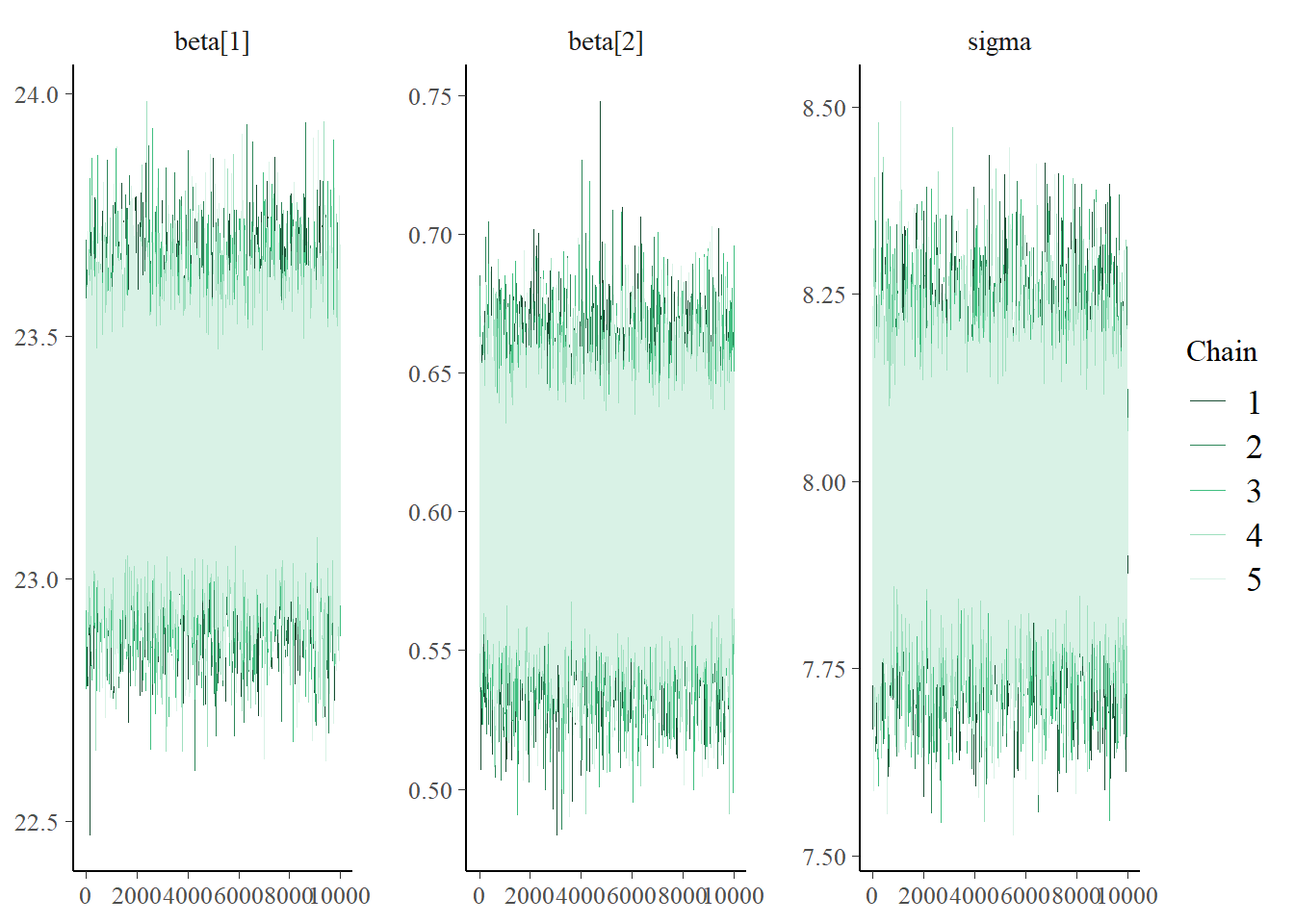

plotPost(beta0)

##               ESS  mean median  mode hdiMass hdiLow hdiHigh compVal pGtCompVal
## Param. Val. 50000 23.28  23.28 23.29    0.95  22.95   23.62      NA         NA
##             ROPElow ROPEhigh pLtROPE pInROPE pGtROPE
## Param. Val.      NA       NA      NA      NA      NA

plotPost(beta1)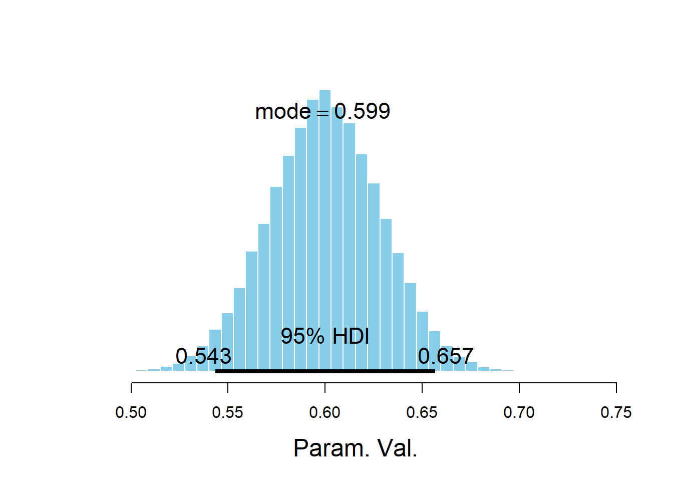

##               ESS   mean median   mode hdiMass hdiLow hdiHigh compVal
## Param. Val. 50000 0.6001    0.6 0.5988    0.95 0.5434  0.6566      NA
##             pGtCompVal ROPElow ROPEhigh pLtROPE pInROPE pGtROPE
## Param. Val.         NA      NA       NA      NA      NA      NA

plotPost(sigma)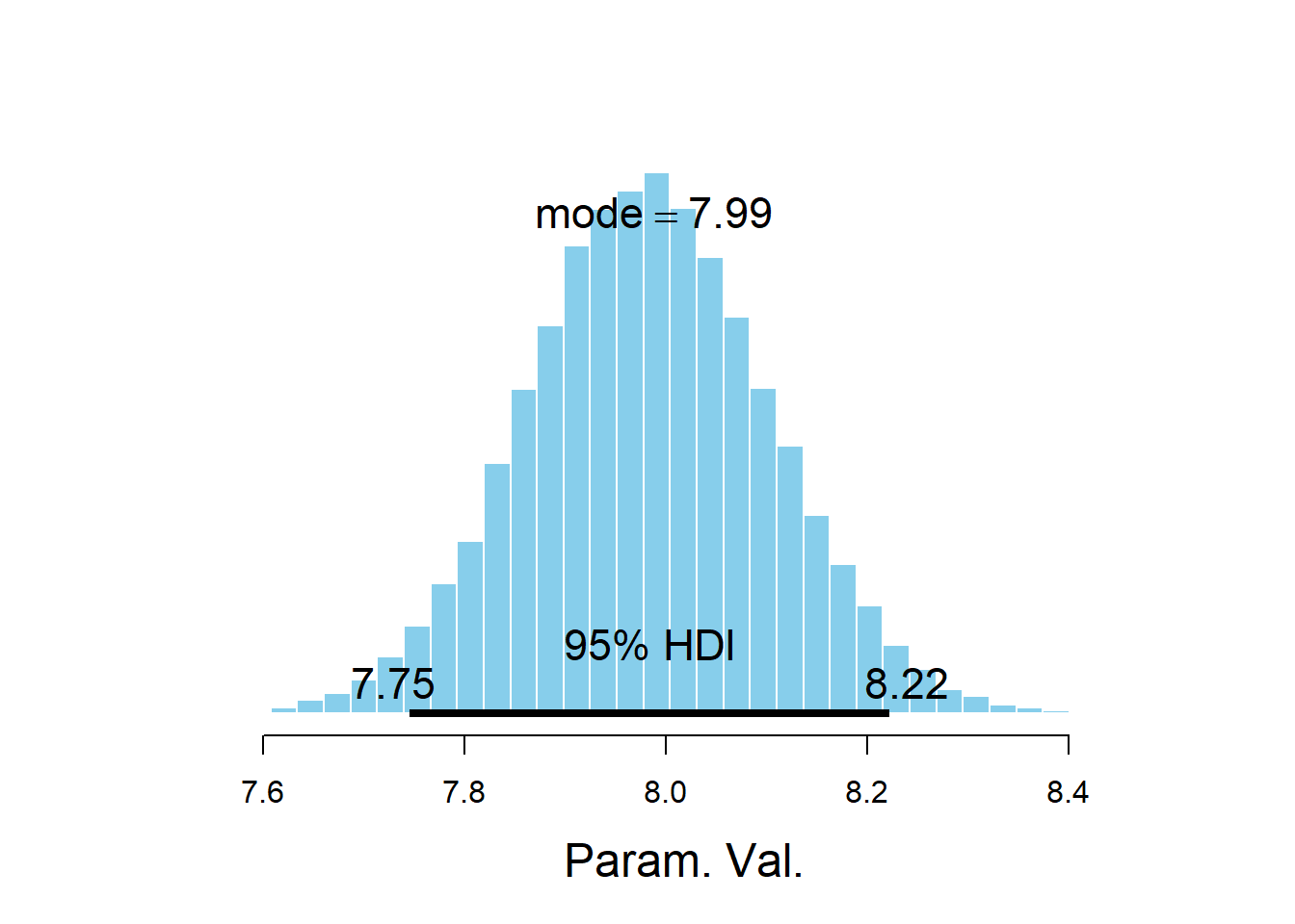

##               ESS  mean median  mode hdiMass hdiLow hdiHigh compVal pGtCompVal
## Param. Val. 30153 7.982  7.981 7.988    0.95  7.746   8.222      NA         NA
##             ROPElow ROPEhigh pLtROPE pInROPE pGtROPE
## Param. Val.      NA       NA      NA      NA      NA

Example 20.4 Now we’ll summarize the posterior distribution and report conclusions.

Find and interpret a 95% posterior credible interval for \(\beta_1\).
Find and interpret a 95% posterior credible interval for the mean PBF for men with a BMI of 15 kg/m².
Find and interpret a 95% posterior credible interval for \(\sigma\).
Find and interpret a 95% posterior predictive interval for men with a BMI of 15 kg/m².
Perform a posterior predictive check of the model by computing posterior predictive intervals for PBF for a variety of values of BMI. Does the model seem reasonable based on the data?

\iffalse{} Solution. to Example 20.4

The posterior distribution of \(\beta_1\), the slope of the population regression line, is approximately Normal with a posterior mean of 0.61 and a posterior SD of 0.03. There is a 95% posterior probability that the slope of the population regression line is between 0.55 and 0.67. That is, there is a posterior probability of 95% that among males, a one kg/\(\text{m}^2\) increase in BMI is associated with between a 0.550 and a 0.669 percentage point increase in percent body fat on average.
```
plot(x,y, xlab = "BMI (kg/m^2)", ylab = "Percent body fat (%)",
 main = paste("Correlation=", cor(x, y)))

nlines = sample(1:length(beta0), 1000)

for (l in nlines){
  abline(beta0[l] - mean(x) * beta1[l], beta1[l], col = "orange", lwd = 1)
}
```
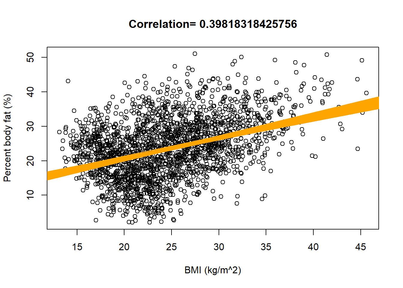
Given the simulated joint posterior distribution of \((\beta_0, \beta_1)\), we can simulate the posterior distribution of \(\beta_0+\beta_1(15-\bar{x})\), the mean PBF for males with a BMI of 15. There is a 95% posterior probability that the mean percent body fat for males with a BMI of kg/\(\text{m}^2\) is between 17.02% and 18.33%.
```
mu_15 = beta0 + beta1 * (15 - mean(x))
hist(mu_15)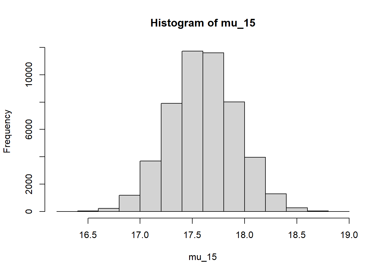
```
```
quantile(mu_15, c(0.025, 0.975))
```
```
##  2.5% 97.5% 
## 16.97 18.23
```
The posterior distribution of \(\sigma\) is approximately Normal with mean 7.99 and SD 0.12. There is a 95% posterior probability that \(\sigma\), which measures the SD of percent body fat among males with the same BMI, is between 7.76 and 8.23 percent.
Simulate values of \(\beta_0, \beta_1, \sigma\) from their joint posterior distribution, then given these values simulate a value of \(y\) from a Normal distribution with mean \(\beta_0+\beta_1(15-\bar{x})\) and SD \(\sigma\). There is a posterior predictive probability of 95% that the PBF of a male with a BMI of 15 kg/m² is between 2.0 and 33.3 percent. Roughly, 95% of males with BMI of 15 kg/m² have percent body fat between 2.00% and 33.3%.
```
xnew = 15
ynew = beta0 + beta1 * (xnew - mean(x)) + sigma * rnorm(50000, 0, 1)
hist(ynew, freq = FALSE, main = paste("Mean=", mean(ynew), ", SD=", sd(ynew)))
lines(density(ynew))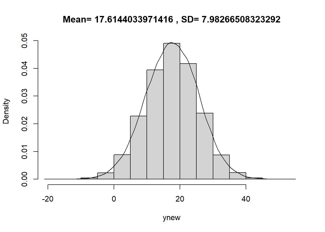
```
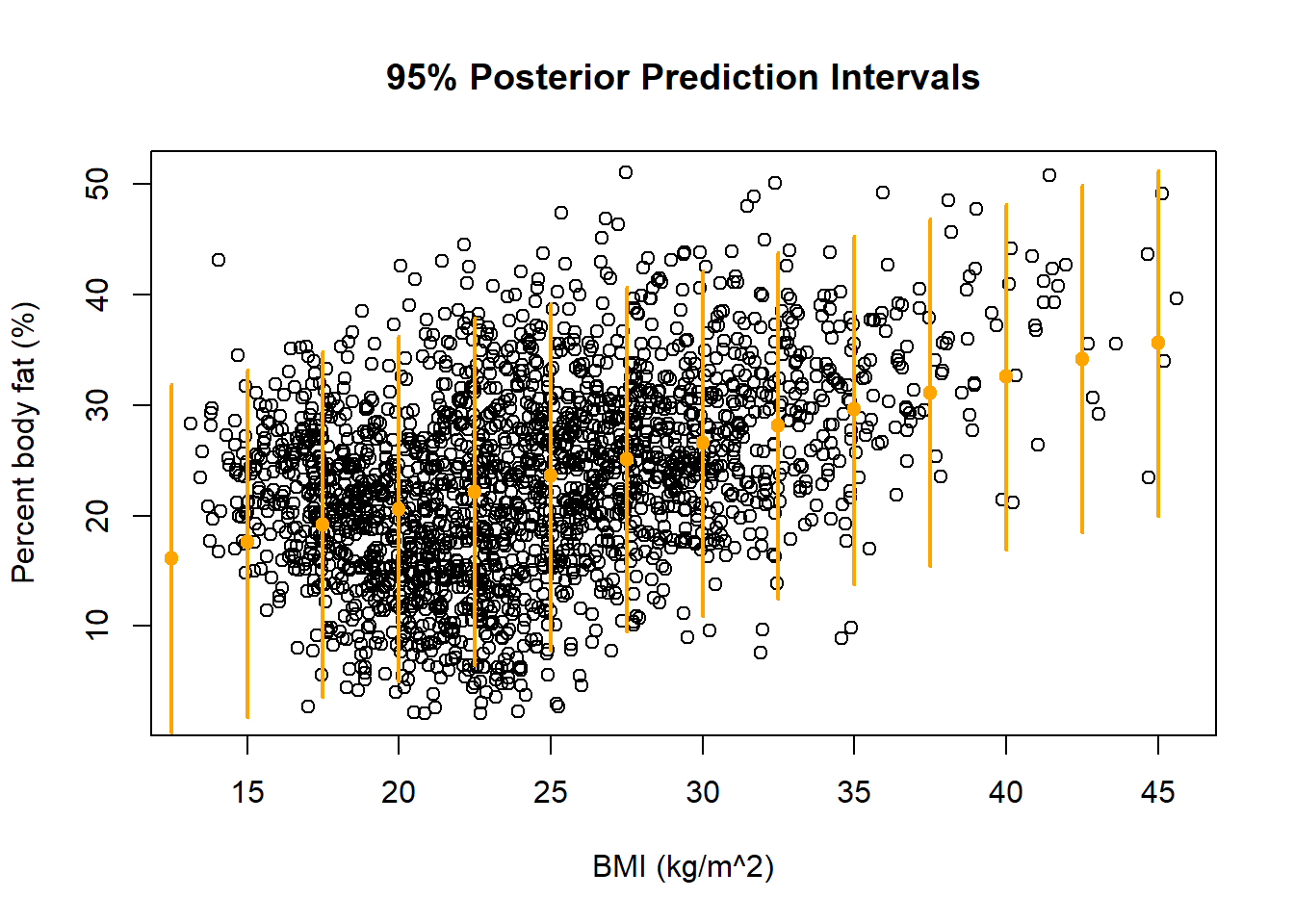
```
quantile(ynew, c(0.025, 0.975))
```
```
##   2.5%  97.5% 
##  1.807 33.159
```
See the plot below. Most of the observed values of PBF fall within the predictive intervals. The model seems reasonable.

plot(x, y, xlab = "BMI (kg/m^2)", ylab = "Percent body fat (%)",
     main = "95% Posterior Prediction Intervals")

xnew = seq(10, 50, 2.5)

for (xx in xnew){
  ynew = beta0 + beta1 * (xx - mean(x)) + sigma * rnorm(50000, 0, 1)
  segments(x0 = xx, y0 = quantile(ynew, 0.025), x1 = xx,
           y1 = quantile(ynew, 0.975), col = "orange", lwd=2)
  points(x = xx, y = mean(ynew), pch = 19, col = "orange")
}

Example 20.5 Now we’ll perform a frequentist simple linear regression model for comparison

Find and interpret the slope of the fitted regression line.
Find and interpret a 95% confidence interval for the slope of the regression line.
Find the equation of the fitted regression line.
Find and interpret the fitted value for men with a BMI of 15 kg/m².
Find and interpret a 95% confidence interval based on the fitted value for men with a BMI of 15 kg/m².
Find and interpret the estimate of \(\sigma\).
Compare the 95% posterior credible intervals with the corresponding frequentist 95% confidence intervals. How are they similar? How are they different?
Find and interpret a 95% prediction interval for men with a BMI of 15 kg/m².
Compare the 95% posterior prediction interval with the corresponding frequentist 95% prediction interval. How are they similar? How are they different?

\iffalse{} Solution. to Example 20.5

Recall that the slope of the fitted (“least squares”) regression line is \[ \frac{rs_y}{s_x} = \frac{\text{correlation}\times\text{SD of response variable}}{\text{SD of explanatory variable}} = \frac{0.398\times 8.7}{5.69} = 0.609 \] Among males, a one kg/\(\text{m}^2\) increase in BMI is associated with a 0.609 percentage point increase in percent body fat on average. (“Percentage points” are the measurement units of percent body fat.)

plot(x, y, xlab = "BMI (kg/m^2)", ylab = "Percent body fat (%)", main = paste("Correlation=", cor(x, y)))

lm1 = lm(y ~ x)
abline(lm1, col = "orange", lwd = 2)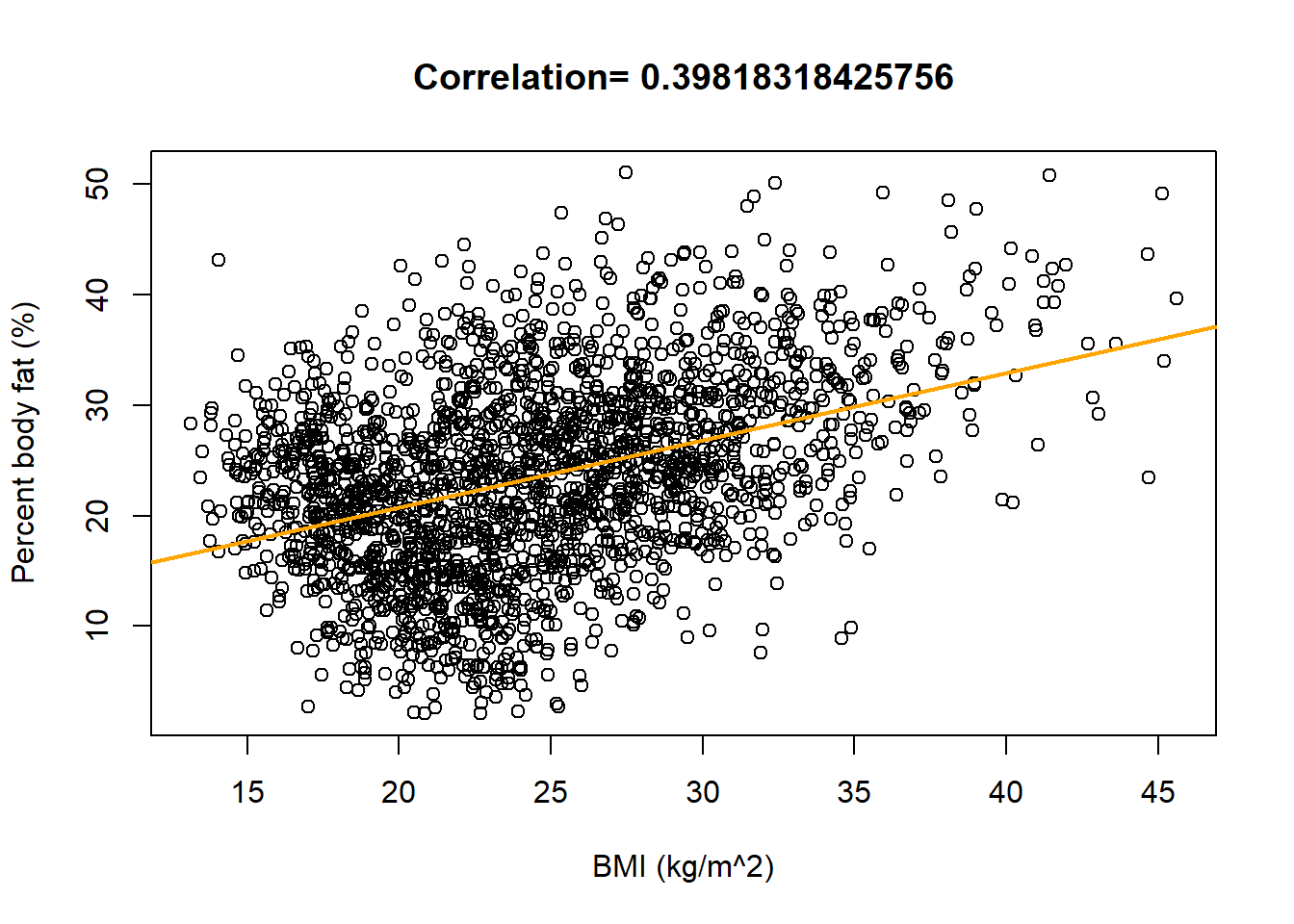

summary(lm1)

## 
## Call:
## lm(formula = y ~ x)
## 
## Residuals:
##    Min     1Q Median     3Q    Max 
## -21.22  -5.52   0.23   5.42  26.00 
## 
## Coefficients:
##             Estimate Std. Error t value            Pr(>|t|)    
## (Intercept)   8.5344     0.7591    11.2 <0.0000000000000002 ***
## x             0.6093     0.0302    20.1 <0.0000000000000002 ***
## ---
## Signif. codes:  0 '***' 0.001 '**' 0.01 '*' 0.05 '.' 0.1 ' ' 1
## 
## Residual standard error: 7.99 on 2155 degrees of freedom
## Multiple R-squared:  0.159,  Adjusted R-squared:  0.158 
## F-statistic:  406 on 1 and 2155 DF,  p-value: <0.0000000000000002

The SE of the slope is 0.03 so a 95% confidence interval has endpoints \(0.609 \pm 2 \times 0.030\). We estimate with 95% confidence that among males, a one kg/\(\text{m}^2\) increase in BMI is associated with between a 0.550 and a 0.669 percentage point increase in percent body fat on average.
```
confint(lm1)
```
```
##             2.5 %  97.5 %
## (Intercept) 7.046 10.0229
## x           0.550  0.6686
```
The slope is 0.609. The intercept is \[ \text{Intercept} = \bar{y} - \text{slope}\times \bar{x} = 23.43 - 0.609 \times 24.45 = 8.534 \] The equation of the regression line is \[ \widehat{\text{Percent body fat (%)}} = 8.534 + 0.609\times \text{BMI(kg/m^2)} \]

For a BMI of 15.0 kg/\(\text{m}^2\) \[ \widehat{\text{Percent body fat (%)}} = 8.534 + 0.609\times 15.0 = 17.67 \text{ percent} \] The mean percent body fat for males with a BMI of kg/\(\text{m}^2\) is 17.67%.

xnew = data.frame(x = c(15))
predict(lm1, xnew, interval = "confidence", se.fit = TRUE)

## $fit
##     fit   lwr   upr
## 1 17.67 17.02 18.33
## 
## $se.fit
## [1] 0.3335
## 
## $df
## [1] 2155
## 
## $residual.scale
## [1] 7.986

We estimate with 95% confidence that the mean percent body fat for males with a BMI of kg/\(\text{m}^2\) is between 17.02% and 18.33%.
The “residual standard error” of \(s=7.99\) percent is an estimate of \(\sigma\). This value measures the variability of percent body fat among males with the same BMI. Roughly, \(s\approx s_Y\sqrt{1-r^2}=8.7\sqrt{1-0.398^2}=7.99\). There is less variability in percent body fat among males with the same BMI, than among men in general.
The values are similar to the frequentist analysis, but the interpretation is different.
Assuming that percent body fats of males with a BMI of 15 kg/m² follow a Normal distribution, with mean 17.67 and standard deviation 7.99, 95% of values lie in the interval with endpoints⁴³ \(17.67\pm2\times 7.99\). We estimate that 95% of males with BMI of 15 kg/m² have percent body fat between 2.00% and 33.35%.
```
predict(lm1, xnew, interval = "prediction")
```
```
##     fit   lwr   upr
## 1 17.67 1.999 33.35
```
Again, the values are very similar to the frequentist analysis. The interpretation of predictions about \(y\) is roughly the same between Bayesian and frequentist, but the uncertainty in the values of \(\beta_0, \beta_1, \sigma\) is accounted for in different ways.

There are a number of ways the assumptions of the simple linear regression model could be revised.

We could assume the mean of \(Y\) changes with \(x\) is a non-linear way (e.g., quadratic).
We could assume distributions other than Normal in the likelihood. For example, we could assume a \(t\)-distribution if outliers were an issue.
We could assume the conditional variance of \(Y\) also changes with \(x\).

Each of the above would be a change in the likelihood, perhaps introducing additional parameters.

We could also combine regression with a hierarchical set up. For example, suppose that the cohort of men in the sample was observed over a ten year period, and BMI and percent body fat was recorded for each man in each year. Then the independence assumption of the simple linear regression model would be violated. However, we could revise the model so that each man had a slope and and intercept relating BMI and PBF, and then fit a hiearchical model.