5.7 Plotting tidal streams

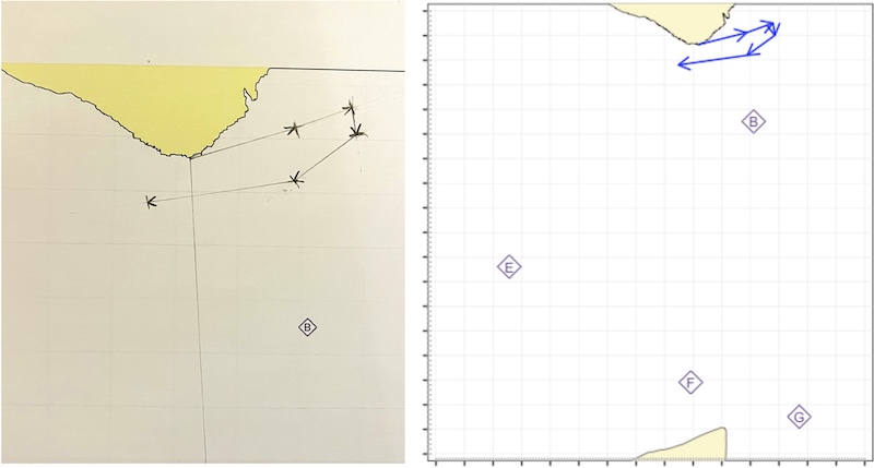
Now we’ve determined the tidal streams for each hour of the crossing, we plot the tidal drift for each hour of the crossing onto our chart. We plot the tidal vectors end to end, reflecting the fact that we expect the tidal drifts to occur sequentially through the crossing:

At this stage, we can see the aggregate effect of our tidal drift through the crossing. In the example above, it’s somewhat to the south. This might be ideal if our crossing heads SSW, but if we’re planning a directly westerly track, we might want to reconsider the timing of our crossing. In the example above, we might consider leaving an hour later to see if that makes the aggregate effect of the tidal streams less.

In the previous section, we calculated the tidal flow for each hour of our example crossing:

Time (BST)	Bearing	Expected rate August 9th
09:30-10:30	76˚	2.0 kt
10:30-11:30	70˚	1.1 kt
11:30-12:30	172˚	0.5 kt
12:30-13:30	234˚	1.4 kt
13:30-14:30	262˚	2.8 kt

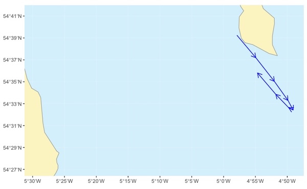
So we’re going to mark a series of arrows:

• For hour 1: at a bearing of 76˚, with a length of 2 nautical miles

• For hour 2: at a bearing of 70˚, with a length of 1.1 nautical miles

etc…

Begin by marking the first hour’s tidal drift: 2 nm at 76˚:

Marking 2 nautical miles of tidal drift at 76˚. 1: set plotter to 76˚. 2: Align plotter to chart north and mark a line at 76˚ from the departure point. 3: Set dividers to 2 nautical miles using latitude scale. 4: Mark 2 nautical miles along the marked line. 5: completed arrow.

Now we mark the remaining hours end to end:

All the tidal drift vector marked on the chart in pencil (left) and on the schematic (right)