10.1 Weighted and Reweighted Least Squares
This technique is another modification of the least squares regression we learned back in the day. “Weighted least squares” is a pretty broad family of techniques, so we’ll start with one particular usage. In this case, the goal is to handle the violation of another (!) regression assumption: constant variance.
10.1.1 Non-constant variance
Here’s some simulated data:
sked.dat = data.frame("x" = runif(100,0,10))
sked.dat = sked.dat %>% mutate("y" = 5 + 2*x + rnorm(100,sd=x))
ggplot(sked.dat) +
  geom_point(aes(x=x, y=y))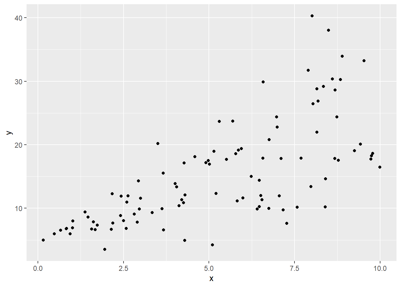
This should immediately catch your eye as violating the constant variance assumption: the vertical spread of the points seems much smaller over at the left, and increasing for larger values of \(x\).
Generally, we would first try to use a variance-stabilizing power transformation on the \(y\) values (that is, taking the log or raising \(y\) to some power, using Tukey’s ladder or Box-Cox to suggest good options). But if that doesn’t work, we have to get into more detail.
Let’s step back and think about the actual problem with non-constant variance: namely, that we spent all that time throwing around a single \(\sigma^2\) value when we were calculating our coefficient estimates, their standard errors (and thus \(t\) statistics and significance), etc. This now seems ill-advised. If the response is really wild and unpredictable (high variance) for certain data points, then we shouldn’t pay as much attention to our observed \(y\)’s at those points. We should give more emphasis to what we see in “reliable areas” – the points for which the response is reliable and well-behaved.
So now, instead of assuming there is a single \(\sigma^2\) value for all points, we allow the idea that there’s a different \(\sigma^2_i\) at each point. How, then, could we estimate these \(\sigma^2_i\)’s? Well, we do have some observed errors.
\[e^2_i\text{ is an estimator of }\sigma^2_{i}\] \[|e_i|\text{ is an estimator of }\sigma_{i}\]
We could use these to estimate \(\sigma^2_i\) (or just \(\sigma_i\)), and then explicitly take that into account when getting our fitted coefficients – by giving points less weight if their error variance is large.
In fact, once we do that, we wind up with a new set of residuals, which we could try to model again, which would lead us to a new set of coefficient estimates… and we could run around this tree until we got to a good answer. This process is called iteratively reweighted least squares (IRLS).
10.1.2 How To Kind of Ignore Things, But Rigorously
Fine, we’ve decided points with a large error variance shouldn’t have as much say in the fit. How do we express “shouldn’t have as much say” mathematically?
We don’t change anything about the dataset – same predictors, same points. Instead, we do something very clever: we change our “goal” when estimating the coefficients.
Let’s go into a bit of detail here. In ordinary least squares, you choose the coefficients to minimize the ordinary least squares criterion. That is, you pick \(b\)’s to minimize the quantity \(Q\), where \[Q=\sum_i(y_i - \beta_0 -\beta_1 x_{i1} - \dots - \beta_{k} x_{i~k})^2\]
Lo this was many days ago, but if you recall, we did a whole bunch of geometric arguments and got a system of equations, which we solved for the coefficients \(\boldsymbol{b}\). (You can get the same system of equations with the magic of partial derivatives!)
Notice that every term in this sum – that is, every point in the dataset – was built from the same formula. So a “mistake” or discrepancy between \(y_i\) and \(\hat{y}_i\) “counted the same” regardless of which \(i\) it was. But in weighted least squares, that doesn’t have to be the case!
We’ll still have a quantity \(Q\) that we are trying to minimize, and it’ll still be built by looking at all the residuals. But this time, we can give each point its own weight in the sum, which we’ll call \(w_i\): \[Q=\sum_i w_i(y_i - \beta_0 -\beta_1 x_{i1} - \dots - \beta_{k} x_{i~k})^2\]
Suppose for some \(i\), \(w_i\) is less than 1. Then if we make a mistake for point \(i\), it won’t count that much towards our total \(Q\) (which is the thing we are trying to minimize). So we might be willing to choose a coefficient vector \(\boldsymbol{b}\) that doesn’t do a great job for point \(i\), if it does better on the other observations.
So what does this mean for our coefficient estimates? Well, back in the day, we solved the normal equations and got this expression for the vector of best-fit coefficients:
\[\boldsymbol b = (\boldsymbol X' \boldsymbol X)^{-1}\boldsymbol X'\boldsymbol y\]
Now – and we aren’t about to prove this – you get a different version of the normal equations:
\[\boldsymbol b_{w} = (\boldsymbol X' \boldsymbol W \boldsymbol X)^{-1}\boldsymbol X' \boldsymbol W \boldsymbol y\]
Hey, what would it mean if \(\boldsymbol{W} = \boldsymbol{I}\)? What would happen to the equation for \(\boldsymbol{b}_w\)?
…where \(\boldsymbol{W}\) is the weight matrix. It’s a diagonal matrix, where the \(i\)th diagonal entry is the weight associated with point \(i\). That is, \(\boldsymbol{W}_{ii} = w_i\).
10.1.3 IRLS for non-constant variance
So let’s hop back to the non-constant variance context: we’d specifically like to downweight points where the error variance is high. Here’s that simulated dataset again:
set.seed(1)
sked.dat = data.frame("x" = runif(100,0,10))
sked.dat = sked.dat %>% mutate("y" = 5 + 2*x + rnorm(100,sd=x))
ggplot(sked.dat) +
  geom_point(aes(x=x, y=y))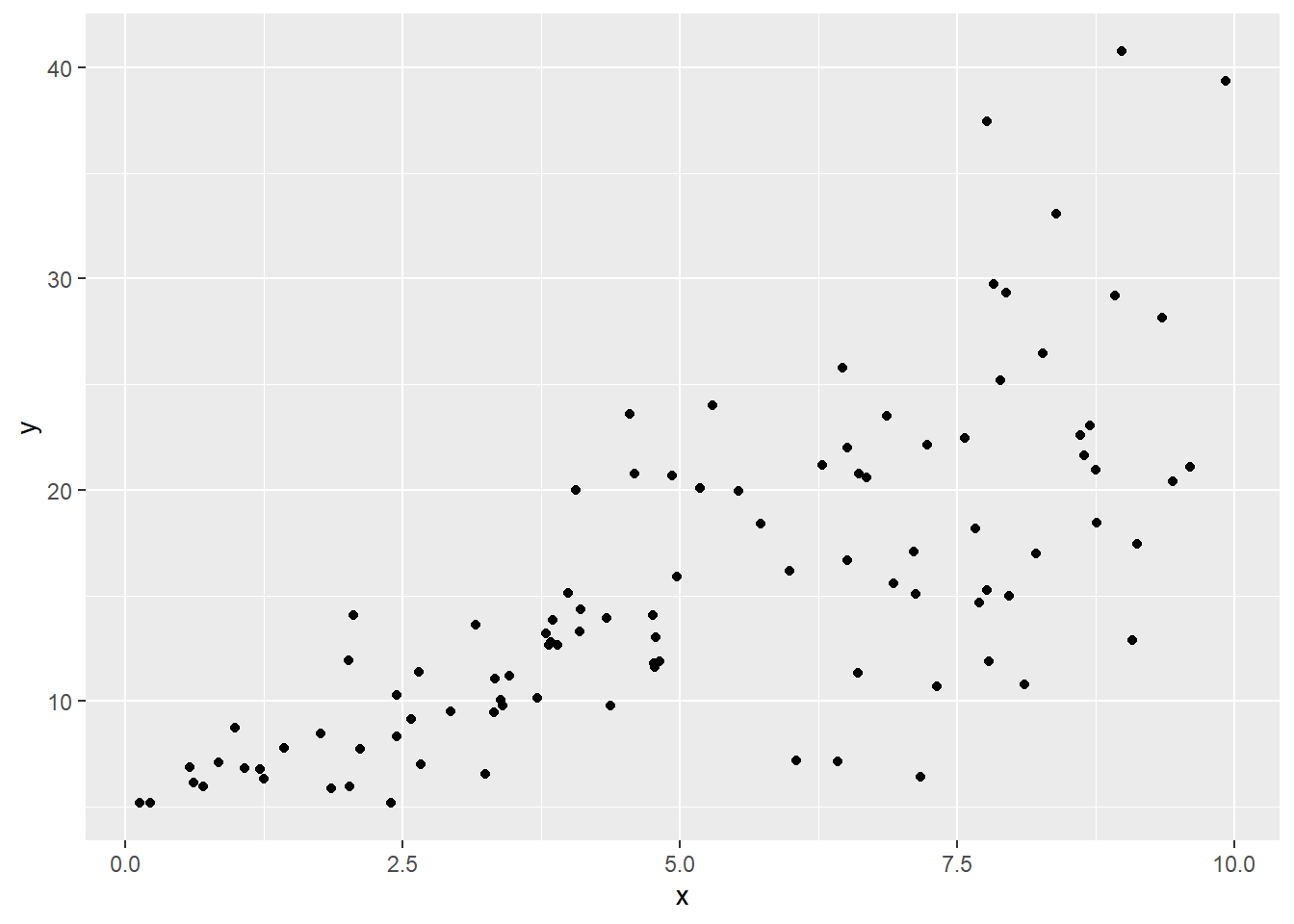
Now, as you might expect, if we fit a linear model here, the residuals will show a similar “megaphone” pattern. Here’s a plot of the absolute values of the residuals vs. \(x\), so we can focus on their magnitude, rather than whether they’re positive or negative:
sked.mod1 = lm(y~x, data=sked.dat)
sked.dat = sked.dat %>%
  mutate("abs.resids" = abs(residuals(sked.mod1)))
sked.resid.mod = lm(abs.resids~x, data=sked.dat)
ggplot(sked.dat) +
  geom_point(aes(x=x, y=abs.resids)) +
  geom_abline(aes(intercept=coef(sked.resid.mod)[1],
                  slope=coef(sked.resid.mod)[2]))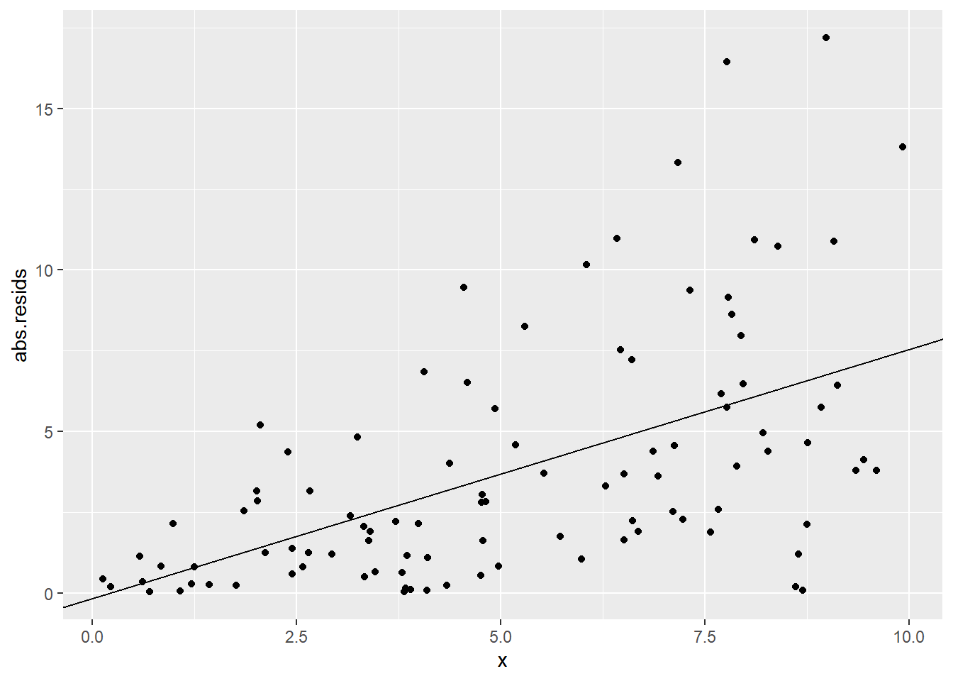
In this classic non-constant-variance situation, it looks like the error variance changes depending on the predictor values. Okay, fine! Let’s make the error variance an actual function of the predictor values.
In particular, let’s suppose that \(\sigma^2_i\) is itself linearly related to (some of) the predictor values for point \(i\). Every point provides its own estimate \(\sigma^2_i\), namely \(e^2_i\). So we could use all of these to try and find the relationship between the relevant \(x\)’s and \(\sigma^2\).
Note that I could either try to model \(e^2_i\) (for \(\sigma^2\)) or just \(|e_i|\) (for \(\sigma\)). It’s kind of up to you, but we’ll use \(|e_i|\) here. This means we are assuming that \(|\sigma_i|\) is a linear function of some predictor(s).
So how does this work?
Step 1: First use ordinary least squares to get some residuals:
\[\boldsymbol e = (\boldsymbol I- \boldsymbol H)\boldsymbol y\]
Step 2: Now, take the absolute value element-wise (you just care how large the residuals are, not which direction); call this vector \(\boldsymbol{e^*}=|\boldsymbol{e}|\). Take any of the predictors that seem to be related to the error variance, and standardize ’em; we’ll call the resulting matrix \(\boldsymbol{Z}\).
Then create a linear regression of \(\boldsymbol{e^*}\) on \(\mathbf{Z}\). This gives you a vector of predicted absolute errors:
\[(\boldsymbol Z' \boldsymbol Z)^{-1}\boldsymbol Z' \boldsymbol e^*\]
Yes, you just did a regression of the estimated absolute error variance on your (standardized) predictors. Life has gotten weird.
These fitted values are \(\hat{s}_i\): they express our estimate of what the error variance should be at each point, assuming it does have that linear relationship to our chosen predictors.
Step 3: Use these fitted values to create weights, downweighting the observations where the estimated error variance is high. Define these weights as \(w_i = \frac{1}{\hat{s}_i}\). Pop them into a weight matrix:
\[\mathbf{W} = \left(\begin{array}{ccccc}w_1&0&0&\cdots&0\\ 0&w_2&0&\cdots&0\\ 0&0&w_3&\cdots&0\\ \vdots&\vdots&\vdots&\ddots&\vdots\\ 0&0&0&\cdots&w_n\\ \end{array}\right)\]
…and use weighted least squares:
\[\boldsymbol b_{w} = (\boldsymbol X' \boldsymbol W \boldsymbol X)^{-1}\boldsymbol X' \boldsymbol W \boldsymbol y\]
Step 4: Now you have new coefficients – and thus new residuals! So you can go around again. Repeat steps 2-4 a few more times to stabilize the coefficients. (They may never completely stop changing, but you or R will have a stopping condition in mind, where you decide they’re really not changing much anymore.)
So what do we get? A fitted regression line – but one that doesn’t pay as much attention to points with larger values of \(x\), because we think that the error variance is larger out there, and our observed values are less reliable.
You can do this kind of model fitting in R with gls() (for “generalized least squares”) in the nlme library. It looks like this:
summary(sked.mod1)##
## Call:
## lm(formula = y ~ x, data = sked.dat)
##
## Residuals:
## Min 1Q Median 3Q Max
## -13.3335 -2.8182 0.0056 2.2465 17.1843
##
## Coefficients:
## Estimate Std. Error t value Pr(>|t|)
## (Intercept) 4.4812 1.1841 3.784 0.000265 ***
## x 2.1254 0.2034 10.451 < 2e-16 ***
## ---
## Signif. codes: 0 '***' 0.001 '**' 0.01 '*' 0.05 '.' 0.1 ' ' 1
##
## Residual standard error: 5.414 on 98 degrees of freedom
## Multiple R-squared: 0.5271, Adjusted R-squared: 0.5223
## F-statistic: 109.2 on 1 and 98 DF, p-value: < 2.2e-16require(nlme)
summary(gls(y~x,weights=varPower(), data=sked.dat))## Generalized least squares fit by REML
## Model: y ~ x
## Data: sked.dat
## AIC BIC logLik
## 572.1908 582.5307 -282.0954
##
## Variance function:
## Structure: Power of variance covariate
## Formula: ~fitted(.)
## Parameter estimates:
## power
## 1.654686
##
## Coefficients:
## Value Std.Error t-value p-value
## (Intercept) 4.849039 0.3418915 14.18298 0
## x 2.028124 0.1315172 15.42098 0
##
## Correlation:
## (Intr)
## x -0.698
##
## Standardized residuals:
## Min Q1 Med Q3 Max
## -2.10973555 -0.64961712 -0.05854267 0.58031505 2.66343574
##
## Residual standard error: 0.0496462
## Degrees of freedom: 100 total; 98 residual