1.1 Categorical Predictors
Thus far, we’ve seen simple linear regression as a way to talk about the linear relationship between two quantitative variables.
As it turns out, that’s a pretty limited view of regression. There are lots of ways to extend the basic principles and techniques to handle other situations and other kinds of data. With those extensions, regression doesn’t have to be simple or linear; you’re not limited to two variables, and none of the variables actually have to be quantitative.
For right now, let’s think about one particular extension: what if we want to predict or explain some quantitative response, using a predictor variable – an \(x\) variable – that’s categorical?
There are lots of situations where you might want to do this. What’s the relationship between a vehicle’s gas mileage and its type – car, truck, SUV? What’s the relationship between salary and gender? Do left-handed batters hit more home runs? And so on.
1.1.1 Example: athlete data
Let’s look at a dataset about Australian athletes. We have several different variables about the physical characteristics of these athletes, each of whom is an elite performer in one particular sport.
Now according to sort of conventional wisdom, different sports tend to encourage different body types: basketball players tend to be very tall, sumo wrestlers are very heavy, and so on. So we might suspect that the BMI, or body mass index, of athletes might vary by sport, and we might be interested in creating a statistical model to tell us how.
To start with, let’s take some performers from gymnastics and water polo (Australians have awesome sports).
athlete_dat = ais %>%
  filter(sport %in% c("Gym", "W_Polo"))
We can make a “scatterplot” of the BMIs for these two groups of athletes:
athlete_dat %>%
  ggplot() +
  geom_point(aes(x = sport, y = bmi))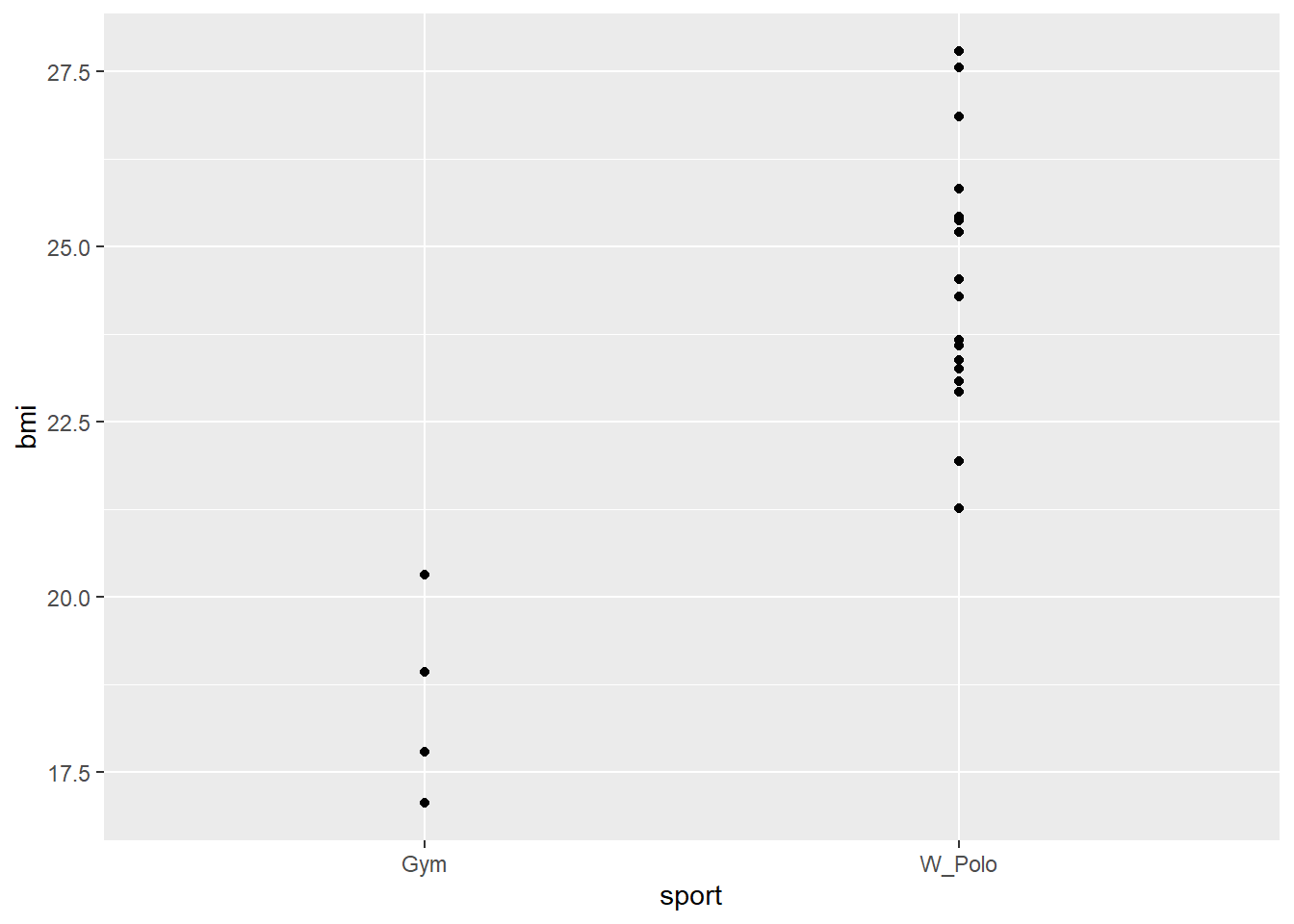
Does seem like there’s a difference! So let’s try and model it.
1.1.2 Encoding a categorical predictor
Okay, so how about a regression equation?
\[\widehat{BMI} = b_0 + b_1{sport}\]
Now, we can find \(b_0\) and \(b_1\) using the dataset. And then to predict a new athlete’s BMI, we’d take their sport, multiply it by \(b_1\), and add \(b_0\).
But, uh. How do you multiply “water polo” by, like, 5?
So we have a conundrum here. The possible values, or levels, of our predictor sport aren’t numbers; they’re “gymnastics” and “water polo.” So if we’re going to create an equation using sport, we need some way to convert these categories or levels into numbers.
These are sometimes referred to as “dummy variables,” but “indicator variables” is preferable if you ask me. It’s more technically precise, it reminds you that the variables are defined using indicator functions, and it doesn’t sound insulting.
The way that we do this is with indicator variables. The name is telling here: such a variable indicates that a particular case is in a particular group. So we could indicate that a given athlete is a water polo player.
Mathematically, we use what’s called an indicator function. This is a function whose value is either 1 or 0 depending on whether something is true or false. We often write indicator functions with the letter I or the number 1, with a subscript to tell us what we’re indicating. So for example:
\[I_{WP} = \begin{cases} 1 & \mbox{ if sport is water polo} \\ 0 & \mbox{ otherwise} \end{cases}\]
Then when we take our model equation:
\[\widehat{BMI} = b_0 + b_1{sport}\]
…we can write it as
\[\widehat{BMI} = b_0 + b_1I_{WP}\]
To predict an athlete’s BMI, we multiply \(b_1\) by either 1 or 0, depending on whether the athlete plays water polo or not; then we add \(b_0\).
Let’s ask R to find the best-fit values for \(b_0\) and \(b_1\):
athlete_lm = lm(bmi ~ sport, data = athlete_dat)
summary(athlete_lm)
##
## Call:
## lm(formula = bmi ~ sport, data = athlete_dat)
##
## Residuals:
## Min 1Q Median 3Q Max
## -3.2065 -1.2165 -0.1865 0.9635 3.3235
##
## Coefficients:
## Estimate Std. Error t value Pr(>|t|)
## (Intercept) 18.5200 0.9009 20.557 1.93e-14 ***
## sportW_Polo 5.9465 1.0013 5.939 1.02e-05 ***
## ---
## Signif. codes: 0 '***' 0.001 '**' 0.01 '*' 0.05 '.' 0.1 ' ' 1
##
## Residual standard error: 1.802 on 19 degrees of freedom
## Multiple R-squared: 0.6499, Adjusted R-squared: 0.6315
## F-statistic: 35.27 on 1 and 19 DF, p-value: 1.023e-05So – with no other information – we’d predict that a water polo player’s BMI is:
18.52 + 5.94 * 1## [1] 24.46…which is actually just the mean BMI for all the water polo players in the dataset:
athlete_dat %>% filter(sport == "W_Polo") %>%
  .$bmi %>% mean()
## [1] 24.46647“But wait!” I hear you say. “What about the gymnasts? There’s the model term \(I_{WP}\), and a line for sportW_Polo in R output, but I don’t see anything about gymnasts.”
Well…what does our equation predict for a gymnast’s BMI?
\[\widehat{BMI} = b_0 + b_1I_{WP}\]
becomes
\[\widehat{BMI} = b_0 + b_1*0\]
…since this person is a gymnast and thus not a water polo player, so \(I_{WP}=0\) for this person.
Plugging in the values from R, we get:
18.52 + 0## [1] 18.52But wait…what’s the mean BMI of the gymnasts in the dataset?
athlete_dat %>% filter(sport == "Gym") %>%
  .$bmi %>% mean()
## [1] 18.52That’s where the gymnasts are – they’re actually the default category. The intercept is our prediction for gymnasts – that’s the baseline. But if an athlete is actually a water polo player, we adjust that baseline prediction by adding \(b_1\), 5.94.
This is an important thing to keep in mind when you’re interpreting the coefficients in a regression with a categorical predictor. 5.94 isn’t the prediction for a water polo player’s BMI; it’s the adjustment to the baseline prediction for a water polo player.
1.1.3 Multiple levels
So what if there are more than two levels, or options, in your categorical predictor? After all, gymnastics and water polo are both great sports, but there are a lot of others out there.
Let’s see what happens if we add some more tennis players to the dataset.
athlete_dat2 = ais %>%
  filter(sport %in% c("Gym", "W_Polo", "Tennis"))
athlete_lm2 = lm(bmi ~ sport, data = athlete_dat2)
summary(athlete_lm2)##
## Call:
## lm(formula = bmi ~ sport, data = athlete_dat2)
##
## Residuals:
## Min 1Q Median 3Q Max
## -4.045 -1.262 0.019 1.069 4.255
##
## Coefficients:
## Estimate Std. Error t value Pr(>|t|)
## (Intercept) 18.520 1.027 18.034 < 2e-16 ***
## sportTennis 2.585 1.199 2.156 0.0395 *
## sportW_Polo 5.946 1.141 5.210 1.42e-05 ***
## ---
## Signif. codes: 0 '***' 0.001 '**' 0.01 '*' 0.05 '.' 0.1 ' ' 1
##
## Residual standard error: 2.054 on 29 degrees of freedom
## Multiple R-squared: 0.5514, Adjusted R-squared: 0.5204
## F-statistic: 17.82 on 2 and 29 DF, p-value: 8.964e-06We’ve just added another term to the regression equation to account for the tennis players. In notation, the equation is now:
\[\widehat{BMI} = b_0 + b_1I_{WP} + b_2 I_{Ten}\]
\[\widehat{BMI} = 18.52 + 5.94*I_{WP} + 2.59* I_{Ten}\]
This new term uses the indicator for “Tennis”: it’s equal to 1 for a tennis player and 0 for everyone else.
So for a gymnast,
\[\widehat{BMI} = 18.52 + 5.94*0 + 2.59*0 = 18.52\]
…which is just \(b_0\). For a water polo player,
\[\widehat{BMI} = 18.52 + 5.94*1 + 2.59* 0 = 24.46\]
And for a tennis player,
\[\widehat{BMI} = 18.52 + 5.94*0 + 2.59* 1 = 21.11\]
So as before, the gymnasts are the baseline group. If the athlete is actually a water polo player, we adjust our prediction by adding 5.94 to the baseline; if they’re a tennis player, we add 2.59 to the baseline instead.
It’s easy to lose track, but always make sure you know what the baseline group is. For example, suppose we throw some field athletes into the dataset as well – shotput, javelin, long jump, that kind of thing.
athlete_dat3 = ais %>%
  filter(sport %in% c("Gym", "W_Polo", "Tennis", "Field"))
athlete_lm3 = lm(bmi ~ sport, data = athlete_dat3)
summary(athlete_lm3)##
## Call:
## lm(formula = bmi ~ sport, data = athlete_dat3)
##
## Residuals:
## Min 1Q Median 3Q Max
## -7.4195 -1.5032 -0.0355 1.5718 6.8805
##
## Coefficients:
## Estimate Std. Error t value Pr(>|t|)
## (Intercept) 27.5395 0.6878 40.042 < 2e-16 ***
## sportGym -9.0195 1.6492 -5.469 1.70e-06 ***
## sportTennis -6.4340 1.1358 -5.665 8.63e-07 ***
## sportW_Polo -3.0730 1.0008 -3.070 0.00355 **
## ---
## Signif. codes: 0 '***' 0.001 '**' 0.01 '*' 0.05 '.' 0.1 ' ' 1
##
## Residual standard error: 2.998 on 47 degrees of freedom
## Multiple R-squared: 0.513, Adjusted R-squared: 0.4819
## F-statistic: 16.51 on 3 and 47 DF, p-value: 1.838e-07Yikes! Not only is there an extra term, but all the coefficient estimates are different now. Why? Because these coefficients are all relative. They’re all adjustments to the prediction for the baseline category. And that category has changed.
Turns out that by default, R looks at the levels in alphabetical order, and uses the first one as the baseline. So the baseline group is now field athletes, who, what with all the throwing things, tend to be quite strong and sturdy and have higher BMIs. If they’re the baseline, we have to adjust downward for water polo players – or tennis players, or gymnasts. The water polo players’ BMIs haven’t changed, but the coefficient for \(I_{WP}\) has changed because you’re starting from a different baseline.
This is a concept that shows up a lot in statistical modeling, especially when you have multiple terms involved. You can’t just think about the coefficients in isolation; you have to think about how they relate to each other.
Response moment: Suppose I convinced R to treat tennis players as the baseline category (there are ways to do this) and got the fitted regression coefficients accordingly. What would be the intercept? What would be the other “rows” in the table of coefficients? And what would be the sign (positive or negative) of each estimated coefficient?