1.9 Regression Assumptions and Conditions (SLR Edition)
Like all the tools we use in this course, and most things in life, linear regression relies on certain assumptions. The major things to think about in linear regression are:
- Linearity
- Constant variance of errors
- Normality of errors
- Outliers and special points
And if we’re doing inference using this regression, we also need to think about the independence condition (just like in other inference tests!), and whether we got a good representative sample from the population. As before, that assumption is best checked by learning about how the data were collected!
We check whether the other assumptions seem to be met using a combination of mathematical tools, plots, and human judgment.
1.9.1 Linearity
The linearity condition hopefully does not surprise you: it is called linear regression, after all. Like correlation, linear regression can only reflect a straight-line relationship between variables. If your variables have some other kind of relationship, you should not use linear regression to talk about them.
Let’s demonstrate with some good old car data. Suppose we want to do a regression of the car’s mileage on its horsepower:
mileage_lm = lm(mpg ~ hp, data = mtcars)
mileage_lm %>% summary()
##
## Call:
## lm(formula = mpg ~ hp, data = mtcars)
##
## Residuals:
## Min 1Q Median 3Q Max
## -5.7121 -2.1122 -0.8854 1.5819 8.2360
##
## Coefficients:
## Estimate Std. Error t value Pr(>|t|)
## (Intercept) 30.09886 1.63392 18.421 < 2e-16 ***
## hp -0.06823 0.01012 -6.742 1.79e-07 ***
## ---
## Signif. codes: 0 '***' 0.001 '**' 0.01 '*' 0.05 '.' 0.1 ' ' 1
##
## Residual standard error: 3.863 on 30 degrees of freedom
## Multiple R-squared: 0.6024, Adjusted R-squared: 0.5892
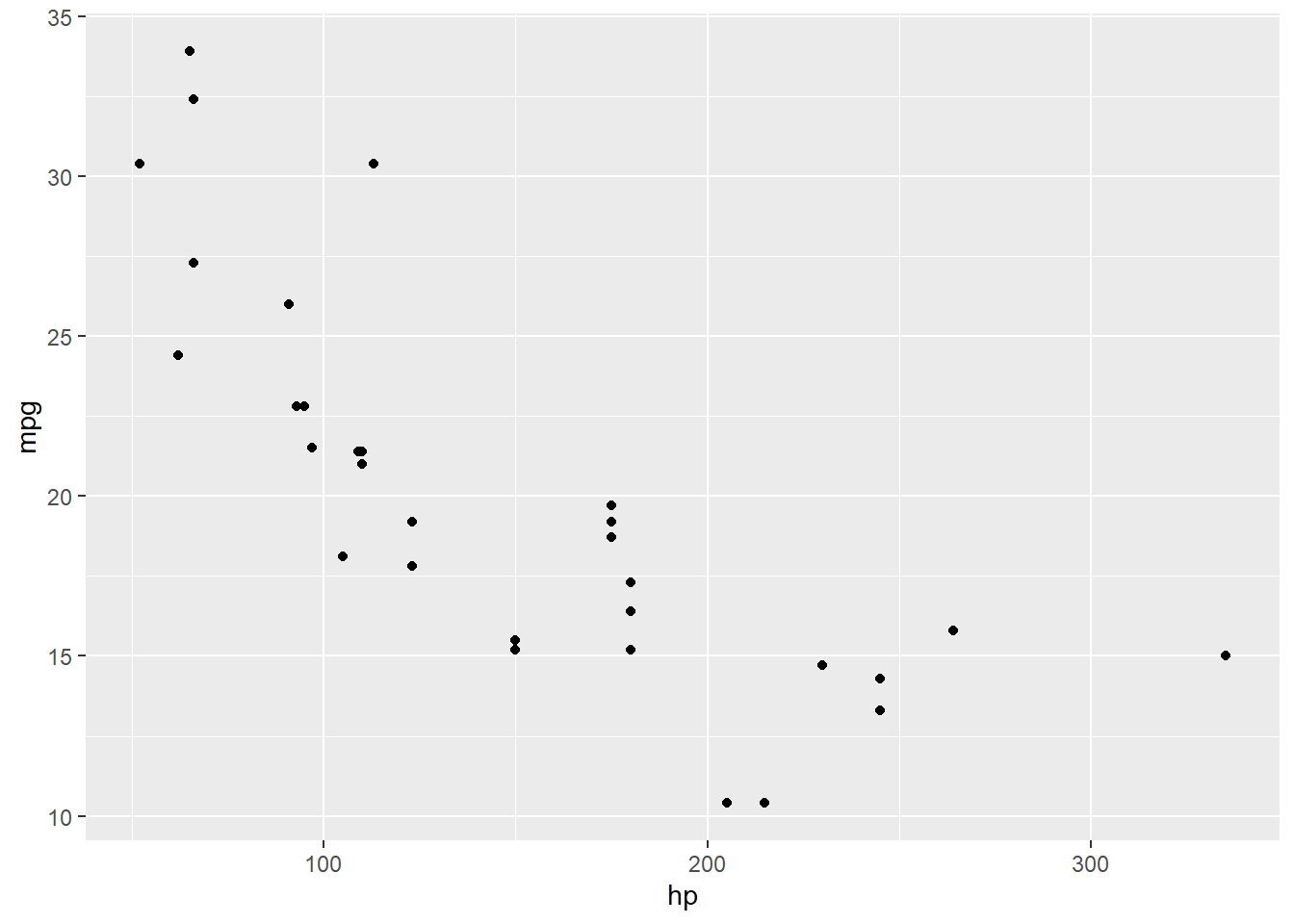
## F-statistic: 45.46 on 1 and 30 DF, p-value: 1.788e-07Okay, cool, fine, looks like there is a negative relationship. But what if we plot the data?
mtcars %>%
  ggplot() +
  geom_point(aes(x = hp, y = mpg))
Oooh huh. Let’s throw the fitted regression line on there for contrast:
mtcars %>%
  ggplot(aes(x = hp, y = mpg)) +
  geom_point() +
  geom_smooth(method = 'lm', se = FALSE)
## `geom_smooth()` using formula 'y ~ x'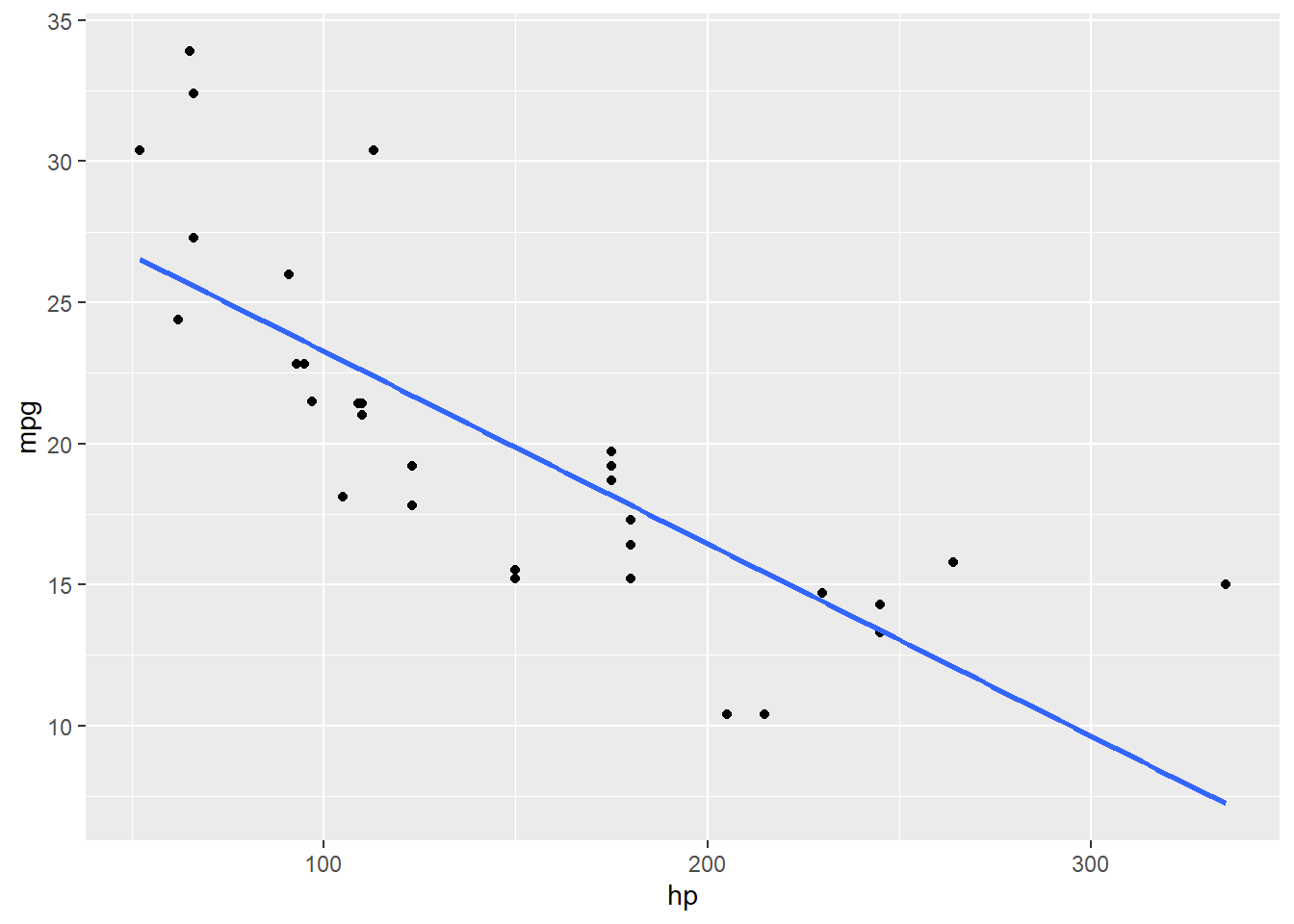
Looks like there is a bend in this relationship – it’s not really a straight line at all.
This can be more obvious if, instead of plotting the original data points, we look directly at the residuals from the regression line. Here, I’m plotting each car’s fitted value, \(\widehat{mpg}\), on the \(x\) axis, and on the \(y\) axis is its residual from this regression line. I’ve also added a horizontal line at 0 – that’s the average of the residuals.
mileage_resid_dat = data.frame(
  "hp" = mtcars$hp,
  "yHat" = mileage_lm$fitted.values,
  "residual" = mileage_lm$residuals
)
mileage_resid_dat %>%
ggplot() +
geom_point(aes(x = yHat, y = residual)) +
geom_hline(aes(yintercept = 0))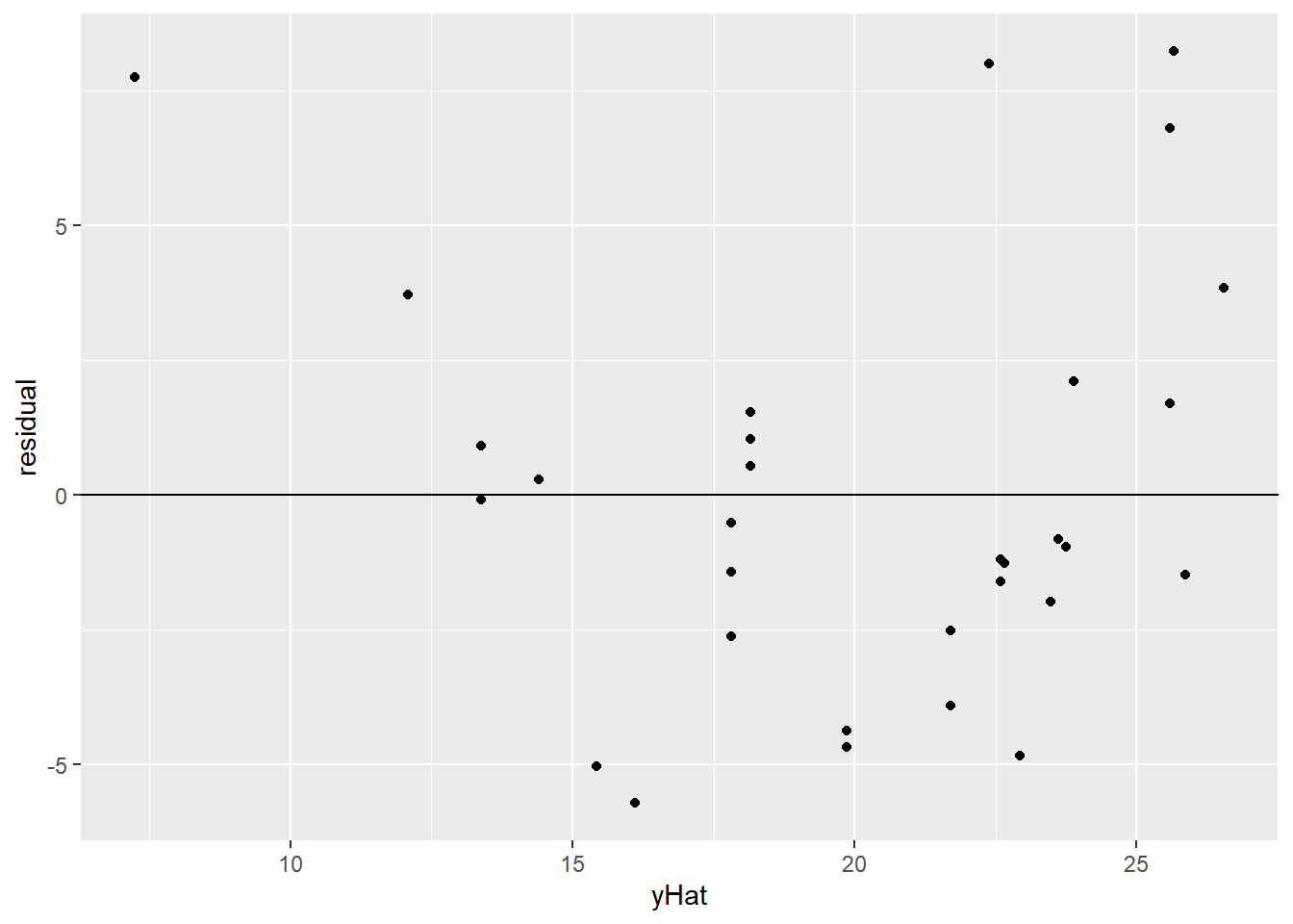
Yeah. So, definitely a bend. First the residuals are mostly positive, then they’re mostly negative, then they’re mostly positive again – as the “cloud” of points bends across the line and back.
This is not a bad kind of question to get used to asking yourself: does what my regression is saying apply equally well throughout the dataset? This principle relates to several of the regression conditions.
So for example, we need linearity because we want our regression slope to describe the \(x\)-vs.-\(y\) relationship for all values of \(x\). If the relationship is curved, then our slope estimate \(b_1\) might actually be right for part of the dataset, but it won’t work elsewhere.
Why does linearity matter? Well, if the relationship isn’t actually linear, then the line is not an accurate or reasonable representation of that relationship. What’s the slope of mileage vs. horsepower? Depends on the horsepower! So that one slope value that we got from our regression fit just isn’t reflecting what’s happening.
1.9.2 Constant error variance
When you fit a model – like a linear regression line – you’ll always have errors. Not all points will fall right on your regression line, no matter how good a line it is. (If the points do all fall on your line, you should worry!)
Now, some of these errors will be positive (the point is higher than the line says it should be) and some will be negative. In fact they’ll average out. But the spread can tell us something about how close the points tend to be to the line. Do we see some errors that are really large, or are they all pretty tightly gathered around 0?
This is all fun and games, but notice the assumption I slipped in there: I talked about “the spread” of the errors – like there is only one spread. But that isn’t always true.
Let’s look at the stopping distances of cars. Here, the predictor \(x\) is the speed the car is going, and the response \(y\) is how far it takes the car to stop. Eyeball this scatterplot. What would you say is the vertical spread of the points – how far they tend to be from the line – if the speed is around 5-10 mph? What if the speed is above 20 mph?
stop_dat = cars
stop_dat %>%
  ggplot() +
  geom_point(aes(x = speed, y = dist))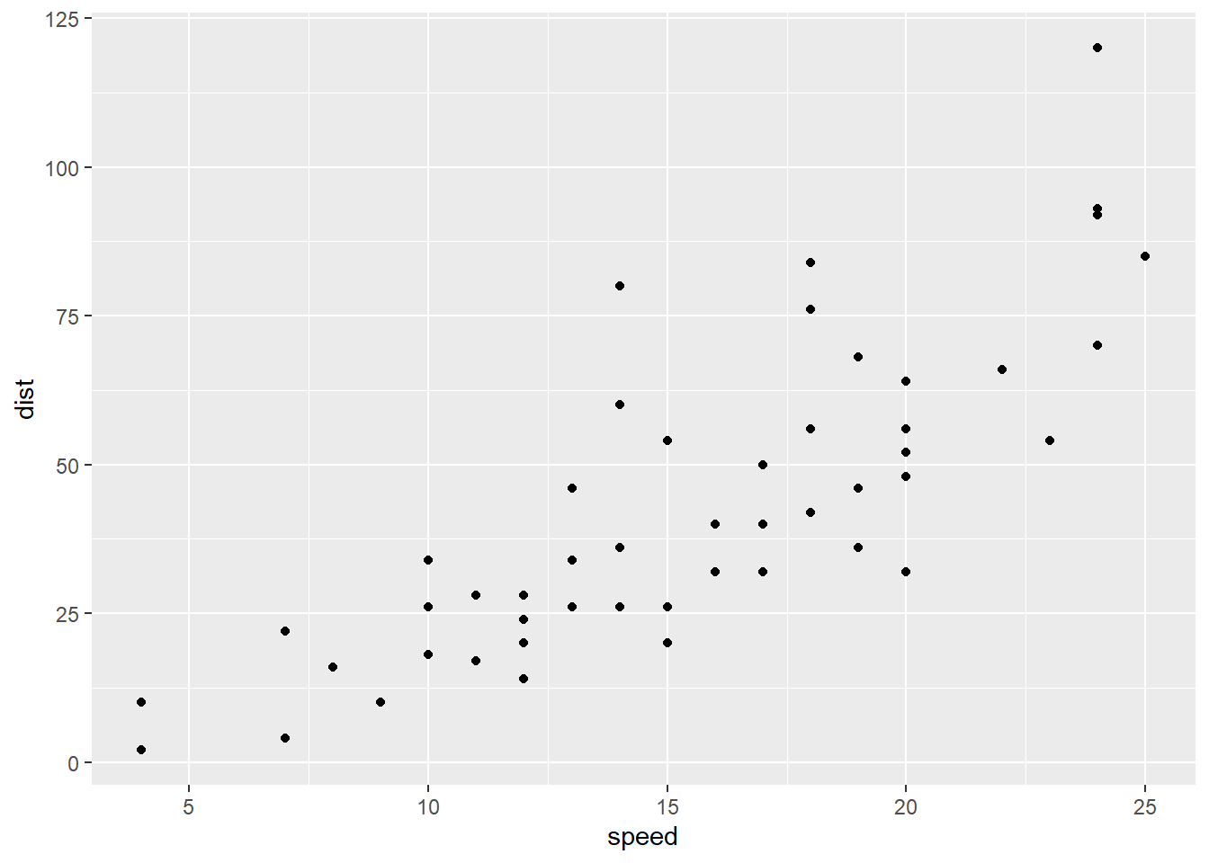
I’m not interested in the exact numbers, but they’re definitely different. It seems like there’s more spread as the values of the \(x\) variable, speed, get higher.
This can be easier to spot if we look at a plot of the residuals vs. the fitted values (\(\widehat{dist}\)). Now there is a definite fan shape happening!
stop_lm = lm(dist ~ speed, data = stop_dat)stop_resid_dat = data.frame(
"speed" = stop_dat$speed,
"yHat" = stop_lm$fitted.values,
"residual" = stop_lm$residuals
)stop_resid_dat %>%
ggplot() +
geom_point(aes(x = yHat, y = residual))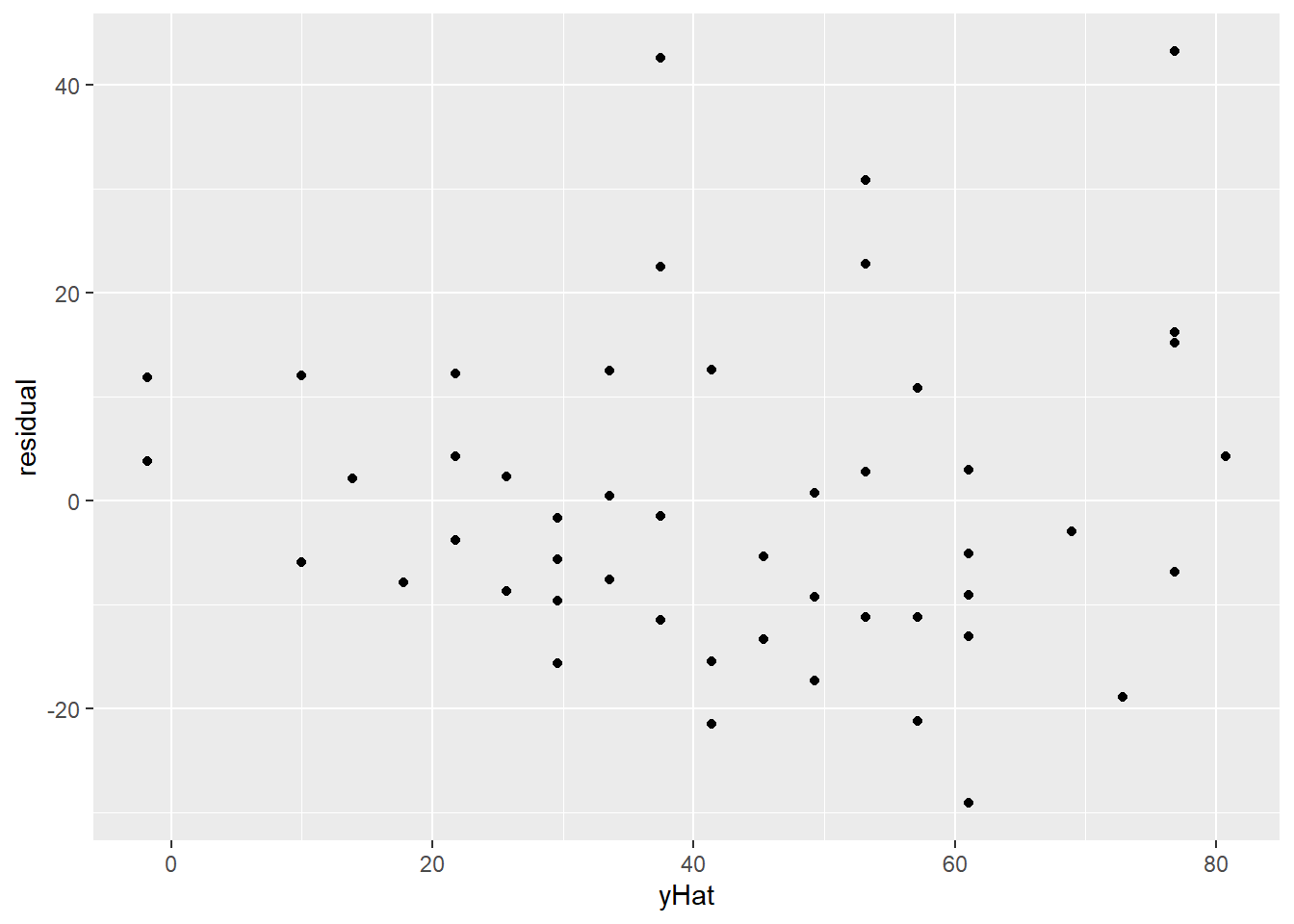
As a side note, R has a built-in plot command for lm objects that will make this plot for you. It’s not as nice-looking or customizable as the ggplot version, but since you’re usually doing this as a quick conditions check, it can be a nice shortcut:
plot(stop_lm, which = 1)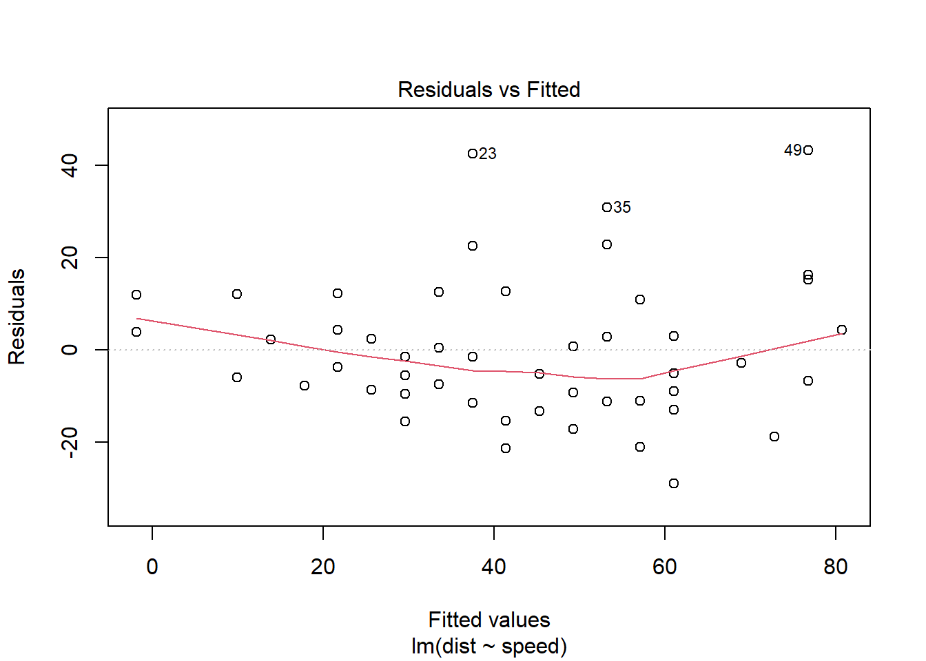
This kind of fan shape is a common form of non-constant variance, but not the only one. You might have fans going the other way, or another shape entirely. What you want is a nice, even spread regardless of the value of the predictor variable.
Similar principle as above! If we have non-constant variance, then our estimate \(s_e\) might be right for part of the dataset, but in other places it will be inaccurate.
Being wrong is part of life, especially statistics. But we don’t want to be wrong in an…unfair way, where we’re accurately modeling one region of the dataset but not others.
Why does constant variance matter? Well, partly that is an exciting mathematical adventure for another time. But at least bear in mind that it doesn’t make sense to talk about the “standard deviation of the residuals,” or \(R^2\), if the residuals don’t always have the same standard deviation!
1.9.3 Normal errors
Linear regression, especially when you start doing inference, also assumes that the errors are Normally distributed. We can check this assumption by looking at the distribution of the residuals. Happily, this isn’t really any different from checking whether any other kind of sample values are Normally distributed. We can check a histogram:
stop_resid_dat %>%
  ggplot() +
  geom_histogram(aes(x = residual), bins = 15)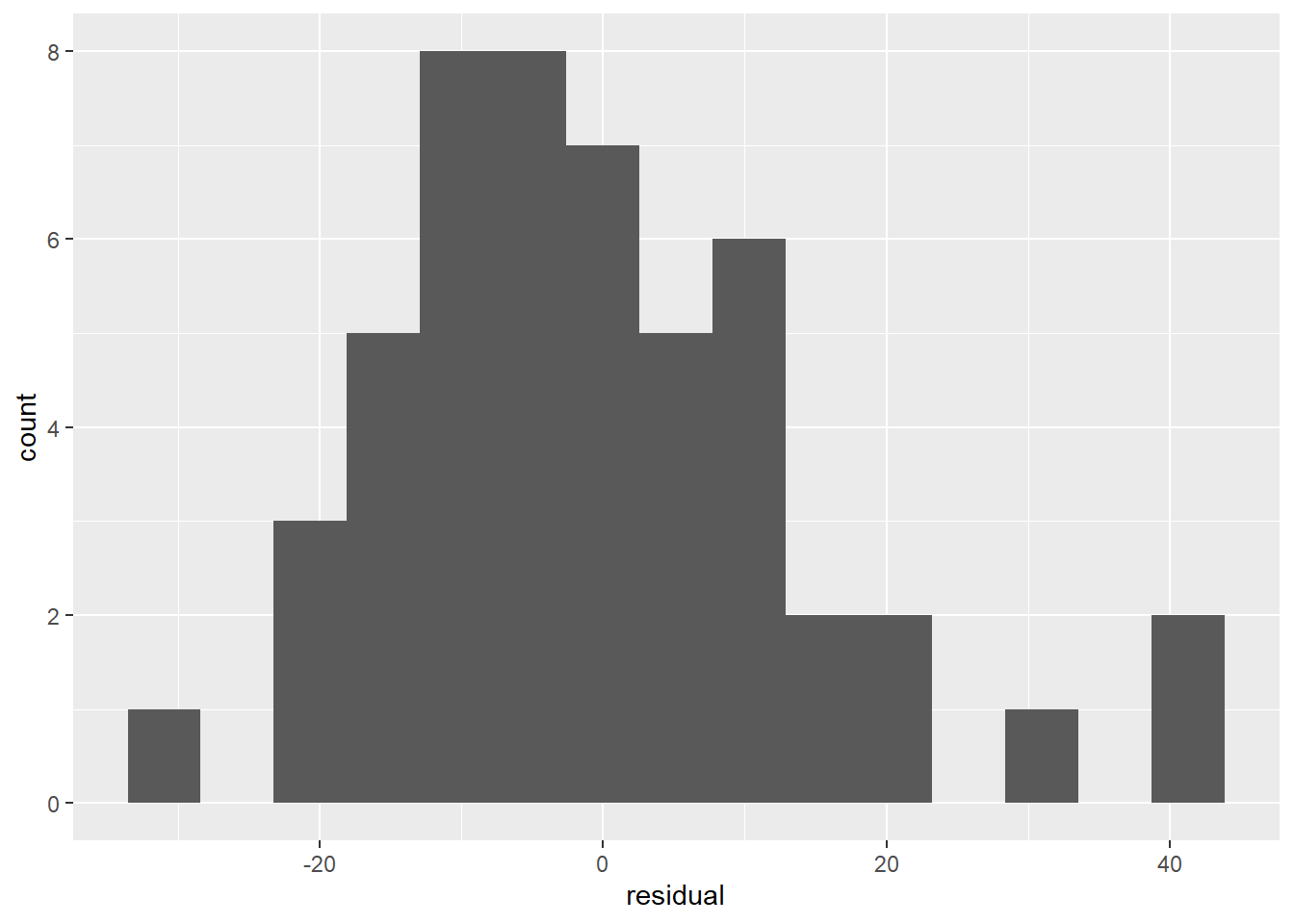
Or a Normal QQ plot:
stop_resid_dat %>%
  ggplot(aes(sample = residual))  +
  stat_qq() +
  stat_qq_line()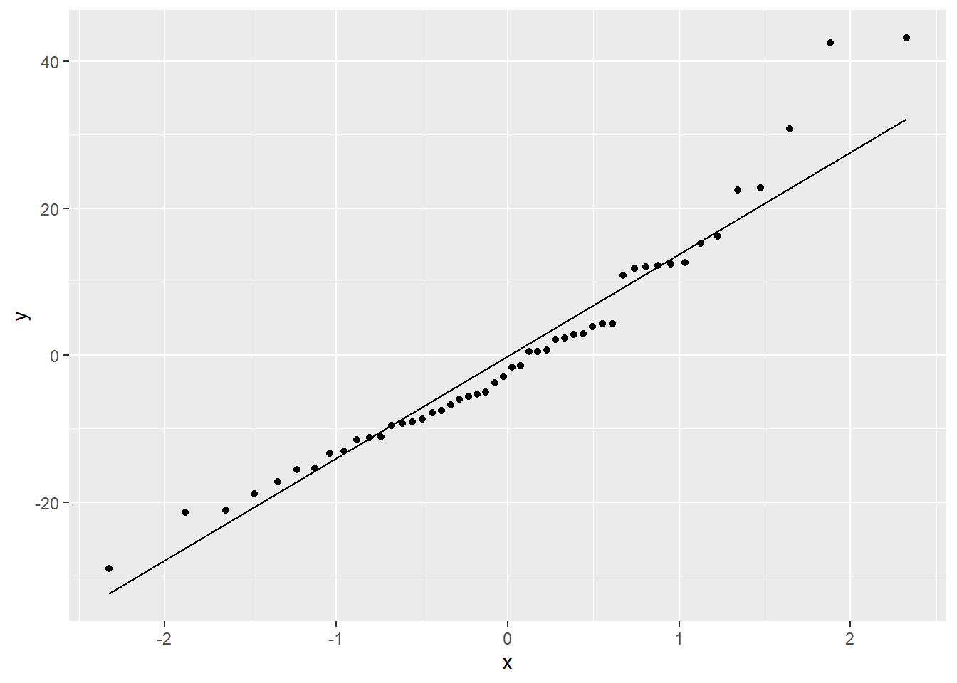
You can also get a less-pretty version of this QQ plot from the lm object. It has the advantage of labeling which cases seem to be extreme, which is handy for going back to the dataset to check them:
plot(stop_lm, which = 2)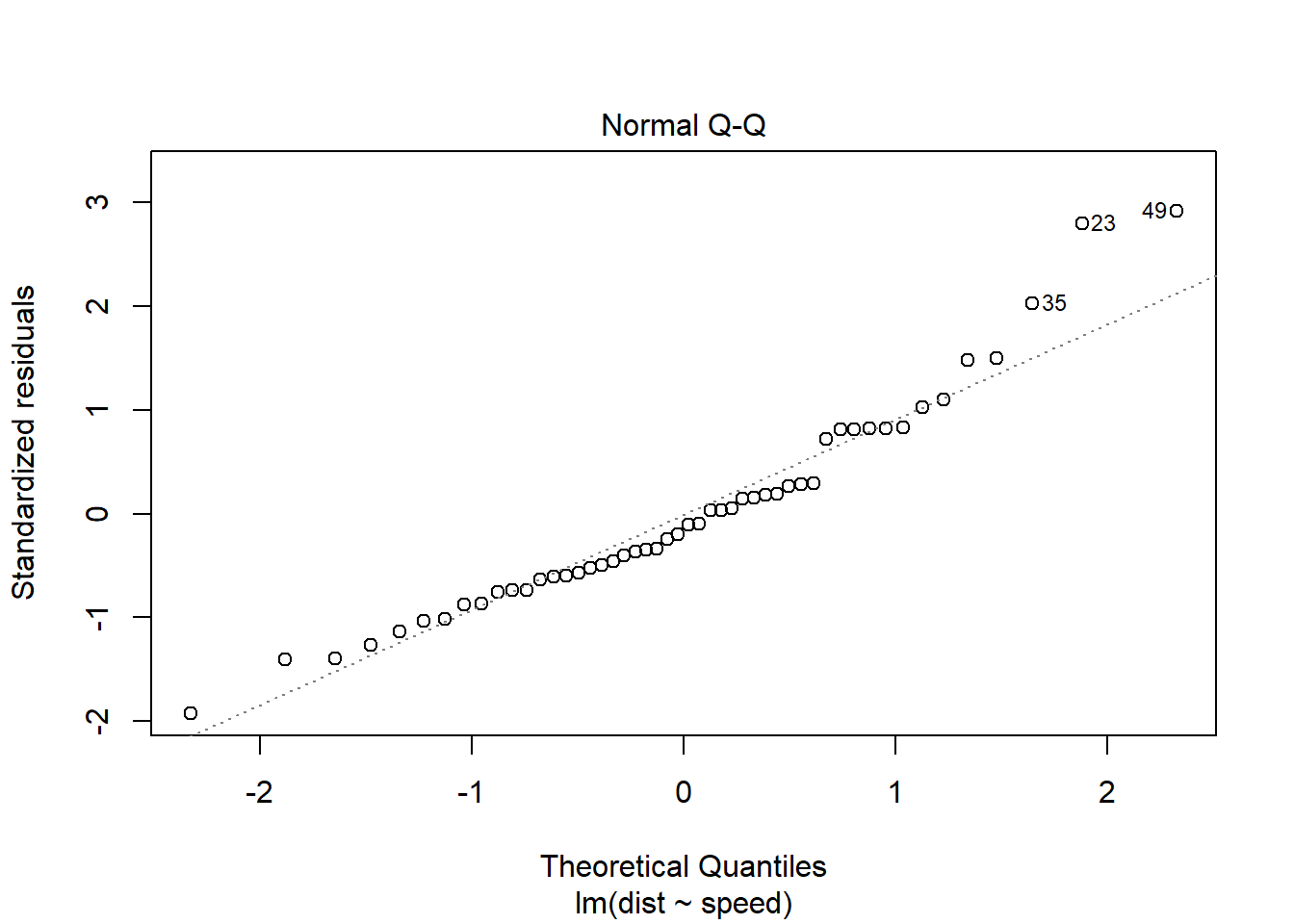
In both the histogram and the QQ plot, there’s a little cause for concern. The histogram looks like it could be a little skewed right – thanks to a handful of really long stopping distances – and the points on the QQ plot have something of a curve, which is also an indication of skew. Plus those really long stopping distances show up again, as points really far off the QQ line.
That said, the Normality assumption isn’t super duper sensitive, so don’t panic if you see a slight deviation from Normality.
Why does Normality of errors matter? Again, partly an adventure for another time. But also, if we want to do inference with regression lines – hypothesis tests and confidence intervals – then we need to have test statistics and null distributions and the whole bit. And all our choices for those things ultimately rely on the errors being Normal.
1.9.4 Transformations
So we’ve now seen some examples where the assumptions for regression are not met. Perhaps you are wondering: what can you do about it?
One answer is to try a transformation of the data – either or both of the variables. The cool thing about transformations is that they can sometimes fix multiple problems at once. For example, a transformation that fixes non-constant variance can also serve to straighten out a nonlinear relationship, and/or make the distribution of errors more Normal.
Now, a transformation that merely shifts the values up or down, or rescales them by multiplying by a constant, won’t help. The most common kind of transformation is a power transformation, where you raise the values to some power: like squaring or taking the square root. Taking the natural log is also very popular.
Let’s try a square-root transformation on the stopping-distance data.
Here’s the original scatterplot:
stop_dat %>%
  ggplot() +
  geom_point(aes(x = speed, y = dist))
And here it is with a square-root transformation applied to the response variable, stopping distance:
stop_dat %>%
  ggplot() +
  geom_point(aes(x = speed, y = sqrt(dist)))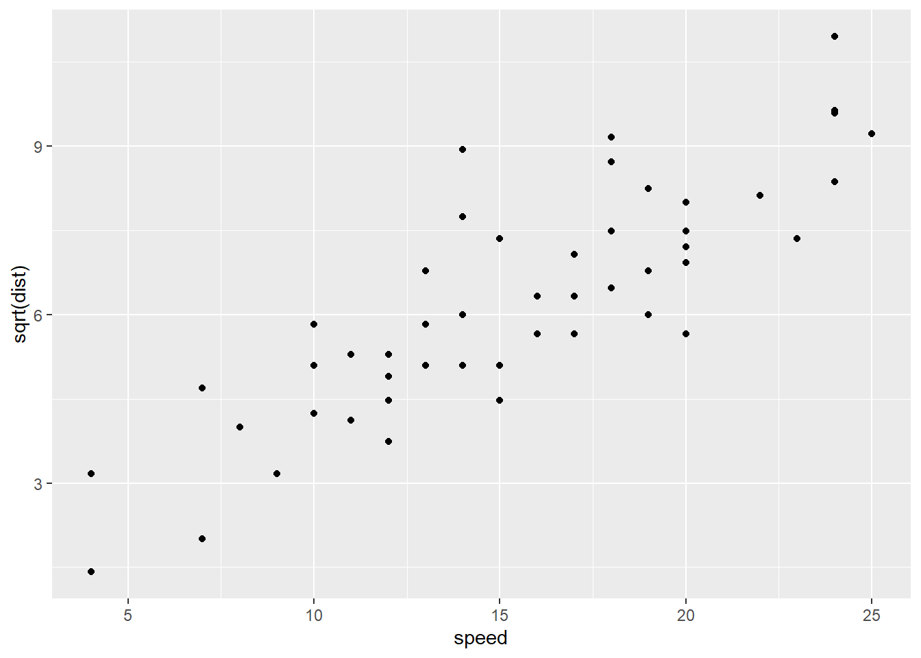
It’s not as easy to see the differences on the original scatterplots, but it does seem like the potential fan shape has been removed, and there’s a possible upward bend in the original data that seems to be gone in the transformed version. Let’s check the residuals:
stop_sqrt_lm = lm(sqrt(dist) ~ speed, data = stop_dat)stop_sqrt_resid_dat = data.frame(
"speed" = stop_dat$speed,
"yHat" = stop_sqrt_lm$fitted.values,
"residual" = stop_sqrt_lm$residuals
)stop_sqrt_resid_dat %>%
ggplot() +
geom_point(aes(x = yHat, y = residual))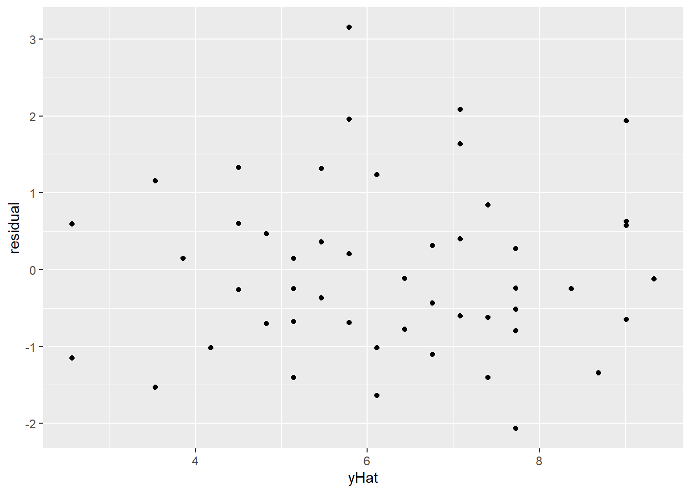
stop_sqrt_resid_dat %>%
  ggplot(aes(sample = residual))  +
  stat_qq() +
  stat_qq_line()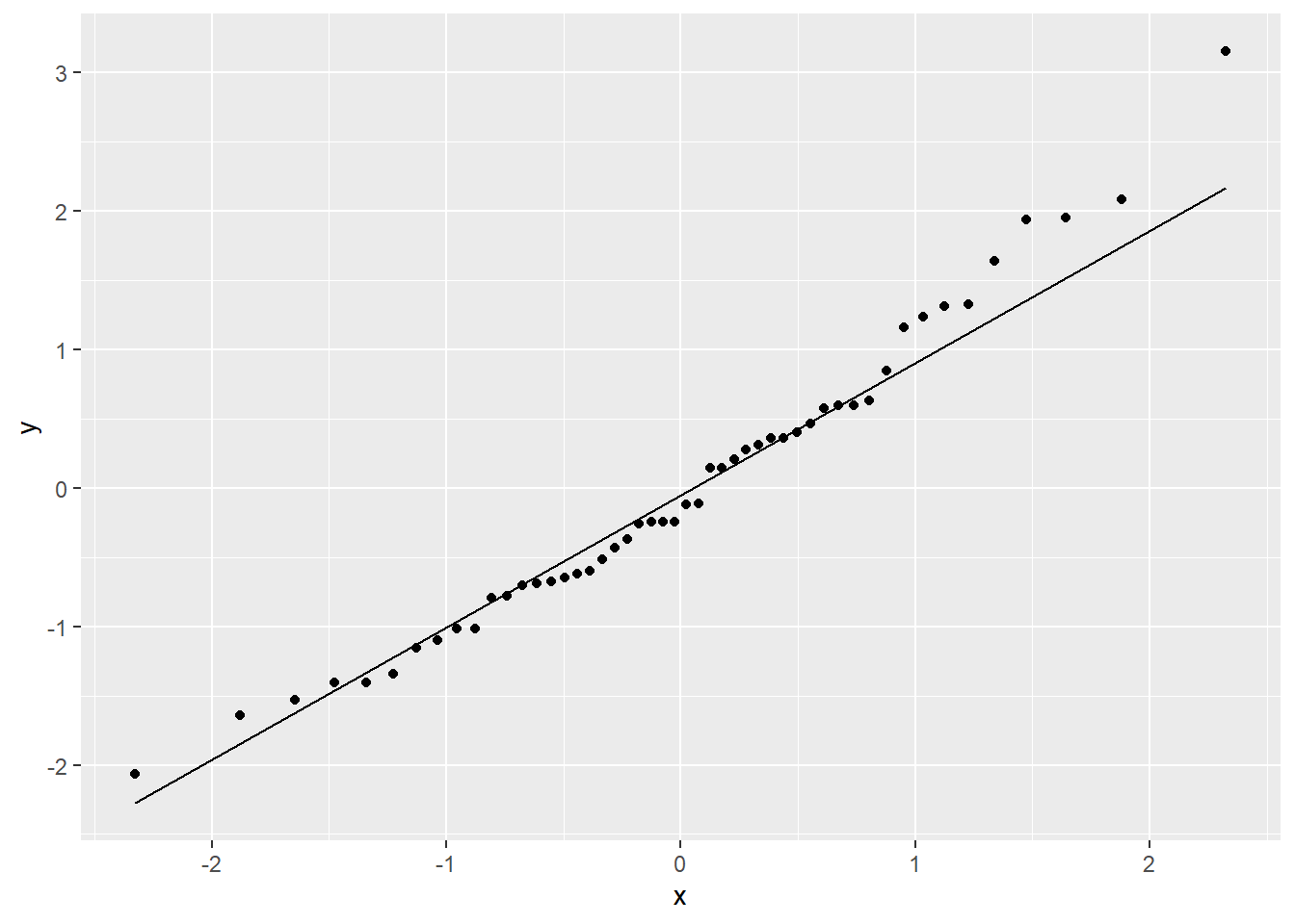
Better! There are still a few outliers, and a very slight bend on the QQ plot, but overall this transformation has gotten us much closer to linearity, constant variance, and Normally distributed errors. So satisfying!
There are some fancy mnemonics for listing transformations you might want to try, like the “ladder of powers” and “Tukey’s circle.” Look them up if you like that kind of thing, but me, I just ask “do I want the big values to get even bigger, or shrink ’em in a bit?” and then I try stuff until something works.
Response moment: What’s a transformation you might want to try on the gas mileage vs. horsepower problem? Here’s the scatterplot:
mtcars %>%
  ggplot() +
  geom_point(aes(x = hp, y = mpg))