1.2 Multiple Linear Regression Fundamentals

1.2.1 The goal of MLR

We had a good time with simple linear regression, right? We could learn all kinds of interesting things.

But sometimes, simple isn’t enough.

It probably won’t surprise you to learn that a lot of things in the real world are complicated. If we want to predict a car’s mileage, or an employee’s salary, or an athlete’s body mass index, we may not be able to do that very well just using one single predictor to make our guess. We could probably do better predicting gas mileage if we looked at the car’s horsepower and its weight rather than either one alone. We could probably predict BMI more effectively if we knew the athlete’s sport and how tall they are. And so on.

Thus: multiple linear regression. We’re still looking at a quantitative response, and looking for linear relationships; but now, we’re looking for linear relationships with multiple predictor variables – all at the same time.

MLR is tremendously common in real-world practice. As is usually the case in statistics, there are all sorts of variations and tweaks and extensions for various circumstances, but even with regular ol’ MLR, you can get a lot done.

1.2.2 The MLR equation

So what does a regression with multiple predictors look like? Well, it looks a lot like a simple linear regression equation…except you tack on some extra terms.

For example, suppose we’re interested in someone’s blood pressure, but we don’t have a blood pressure cuff, so we want to try and predict it based on some other things that are easier to measure.

In a simple linear regression, we might use their pulse rate as a predictor. We’d have the theoretical equation:

\[\widehat{BP} = \beta_0 + \beta_1 Pulse\]

…then fit that to our sample data to get the estimated equation:

\[\widehat{BP} = b_0 + b_1 Pulse\]

According to R, those coefficients are:

bp_simple = lm(BPSysAve ~ Pulse, data = bp_dat)
bp_simple$coefficients

## (Intercept)       Pulse 
##  106.637346    0.163712

But wait! we say. What if we also use the person’s age to help improve our prediction? Well, we can just add another term to the equation:

\[\widehat{BP} = \beta_0 + \beta_1 Pulse + \beta_2 Age\]

Or the estimated version:

\[\widehat{BP} = b_0 + b_1 Pulse + b_2 Age\]

And again, we use R to get these fitted coefficient values:

bp_multi = lm(BPSysAve ~ Pulse + Age, data = bp_dat)
bp_multi$coefficients

## (Intercept)       Pulse         Age 
##  83.3709862   0.2597820   0.3632164

But what does this all mean?

1.2.3 MLR interpretation

There’s one phrase I want you to get really used to here – repeat it to yourself until it really sinks in. It should be basically a reflex when you’re talking about multiple regression. That term is:

…after accounting for other predictors.

When you look at the slope coefficient for some predictor \(x_i\) in your multiple regression, it doesn’t exist in a vacuum. That’s the relationship between \(x_i\) and \(y\) after taking all the other x’s into account.

In our example, we had the fitted model:

\[\widehat{BP} = 97.4 + 0.056 Pulse + 0.414 Age\]

The interpretation of the intercept \(b_0\) is much the same as before: it’s where the line – well, now it’s a high-dimensional line – crosses the \(y\) axis. In context, this is the blood pressure we’d predict for someone with no pulse rate who is 0 years old, which is not actually meaningful. But we’re used to that, with the intercept.

The slope coefficients are, as usual, more interesting. Take \(b_1\), 0.056. For someone with a pulse rate 1 beat per minute faster of the same age, we’d predict that such a person would have a blood pressure 0.056 units higher. That “of the same age” is key! If the new person with the faster pulse has a different age, then our prediction wouldn’t just go up by 0.056; we’d also have to adjust for the new person’s age.

Another way to say this would be: “for people of a given age,” – or “after accounting for age,” – “1 bpm faster pulse rate is associated with, on average, blood pressure 0.056 units higher.”

There are a couple of kind of technical, but very important, pieces to that interpretation. One is the “on average” part. You have to say something like “on average” or “predicted,” because our model is not actually correct for any given person – it’s just describing the overall trend and making a prediction. And the other technical piece is the “after accounting for age.”

Notice the difference in the slope of pulse rate in our two models – one using just pulse alone, and the other using both pulse and age:

bp_simple %>% summary()

## 
## Call:
## lm(formula = BPSysAve ~ Pulse, data = bp_dat)
## 
## Residuals:
##     Min      1Q  Median      3Q     Max 
## -27.354 -10.548  -0.442   7.925  40.301 
## 
## Coefficients:
##             Estimate Std. Error t value Pr(>|t|)    
## (Intercept) 106.6373    12.3179   8.657 2.28e-11 ***
## Pulse         0.1637     0.1650   0.992    0.326    
## ---
## Signif. codes:  0 '***' 0.001 '**' 0.01 '*' 0.05 '.' 0.1 ' ' 1
## 
## Residual standard error: 14.9 on 48 degrees of freedom
## Multiple R-squared:  0.0201, Adjusted R-squared:  -0.0003142 
## F-statistic: 0.9846 on 1 and 48 DF,  p-value: 0.326

bp_multi %>% summary()

## 
## Call:
## lm(formula = BPSysAve ~ Pulse + Age, data = bp_dat)
## 
## Residuals:
##     Min      1Q  Median      3Q     Max 
## -24.268  -9.678  -1.036   8.174  37.295 
## 
## Coefficients:
##             Estimate Std. Error t value Pr(>|t|)    
## (Intercept)  83.3710    12.7404   6.544 4.03e-08 ***
## Pulse         0.2598     0.1498   1.735  0.08937 .  
## Age           0.3632     0.1002   3.624  0.00071 ***
## ---
## Signif. codes:  0 '***' 0.001 '**' 0.01 '*' 0.05 '.' 0.1 ' ' 1
## 
## Residual standard error: 13.31 on 47 degrees of freedom
## Multiple R-squared:  0.2342, Adjusted R-squared:  0.2016 
## F-statistic: 7.185 on 2 and 47 DF,  p-value: 0.001894

When we add age to the model – that is, when we look at pulse rate vs. blood pressure among people of a given age – we see that the slope of pulse is higher, and it even becomes (marginally) significant where it wasn’t before.

Let’s look at what’s happening visually. Here’s a scatterplot of pulse rate and blood pressure:

bp_dat %>%
  ggplot() +
  geom_point(aes(x = Pulse, y = BPSysAve))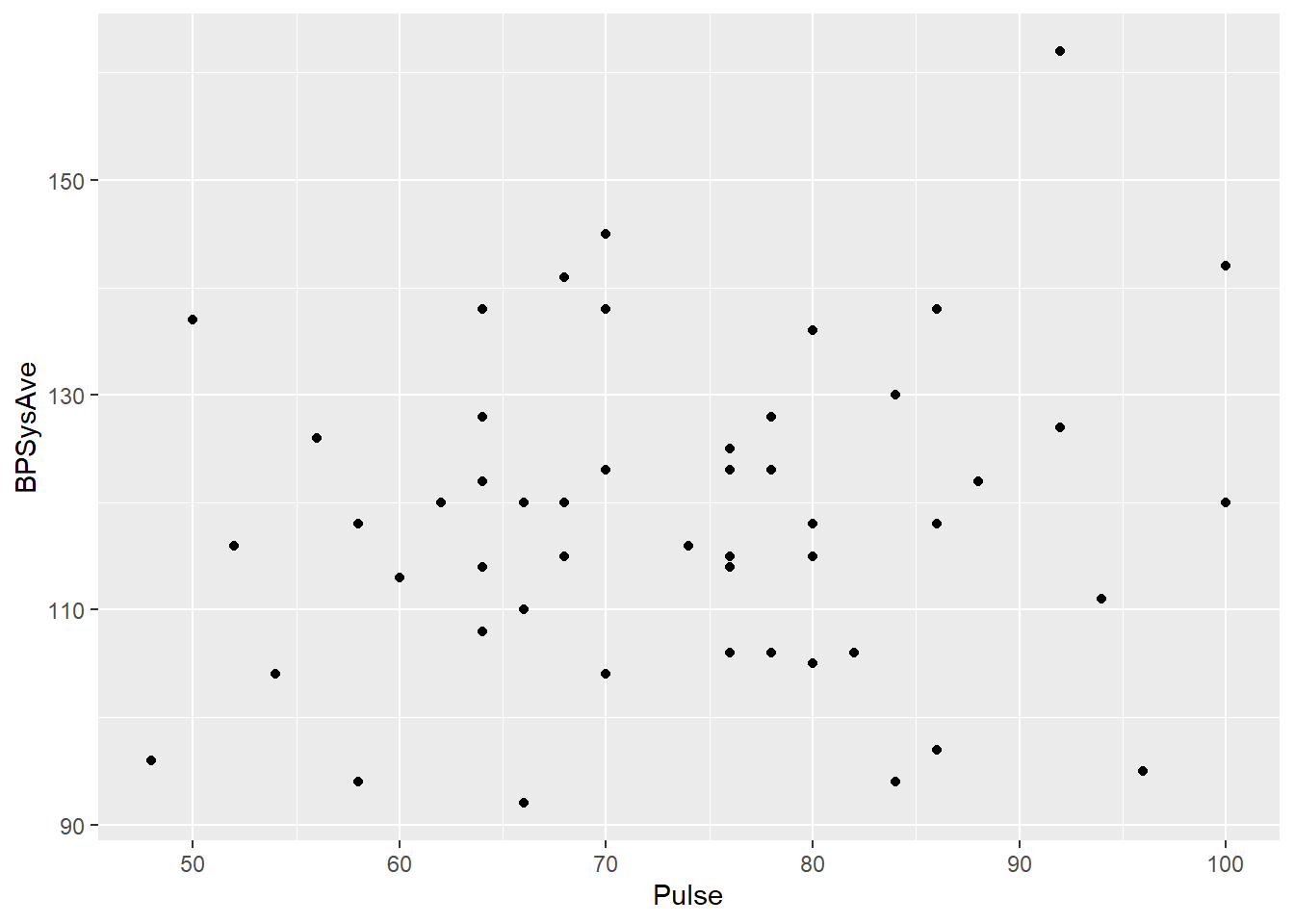

Doesn’t look all that promising. But suppose we just look at people of the same age. We don’t have that many folks who are exactly the same age in this dataset, but let’s look at the ones between 40 and 50:

bp_dat %>%
  ggplot() +
  geom_point(aes(x = Pulse, y = BPSysAve)) +
  geom_point(data = bp_dat %>%
               filter(between(Age, 40, 50)),
             aes(x = Pulse, y = BPSysAve),
             color = "red", size = 2)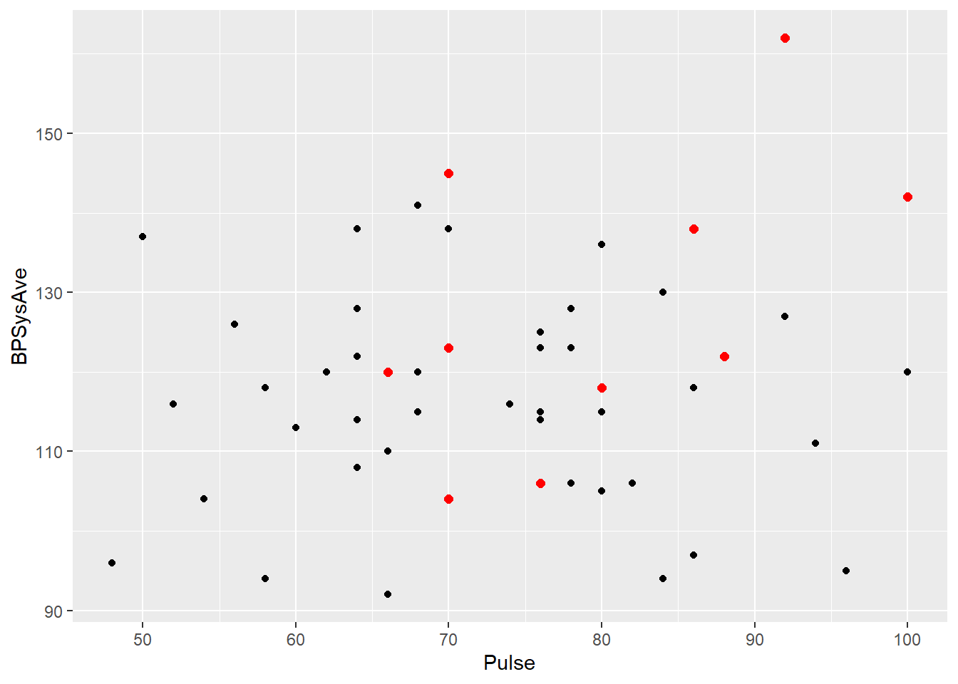

Among those folks, there seems to be a somewhat steeper, maybe even stronger relationship between pulse and blood pressure. So the relationship between pulse and blood pressure overall is different than the relationship after taking age into account.

Response moment: Suppose you call up the local elementary school and get some data on their students: each student’s height and their reading speed, in words per minute. Do you think you will see a relationship between those variables? What would happen if you added the students’ age as another predictor?