4.1 Intro to the t distribution

4.1.1 What’s the goal here?

Getting really deep into the mathematics of the \(t\) distribution is a whole adventure. But as an introduction, I do want to say a little bit about why we sometimes have to use it, and more or less what it looks like.

4.1.2 Why not Normal?

If you’ve done any sort of sampling or inference work, you may have previously noticed a bit of a problem. We keep talking about this \(\sigma\), the population standard deviation. It shows up in the sampling distribution of the sample mean \(\overline{y}\), for example: \[\overline{y}\sim N(\mu, \frac{\sigma}{\sqrt{n}})\] …thanks to the CLT. If we want to talk about how much different samples’ \(\overline{y}\)’s vary – their spread – then we need this standard deviation \(\frac{\sigma}{\sqrt{n}}\), and we just don’t know what it is.

One way of dealing with this is to pretend we know what \(\sigma\) is, by estimating it with our sample standard deviation, \(s\). I mean, that is kind of our best guess, so it’s not a bad idea.

The problem is this: \(s\) isn’t equal to \(\sigma\). We only have a sample, so our estimate is going to be a bit wrong. Interestingly, we know something about how it tends to be wrong: it tends to be too small.

This means that if we say \[\overline{y}\sim N(\mu, \frac{s}{\sqrt{n}})\quad \mbox{<- this is wrong!!}\]

we’ll be underestimating the spread a bit. We’re actually more likely to get extreme \(\overline{y}\) values, far from \(\mu\), than this would indicate.

If we standardize \(\overline{y}\) by subtracting the mean and dividing by \(\frac{s}{\sqrt{n}}\), we don’t get a standard Normal distribution. We get something else – something that’s more likely to have extreme positive or negative values.

4.1.3 What does the \(t\) do?

Yes, Guinness as in the beer! There’s a long and storied history of statisticians working in industry to help with quality assurance, forecasting, and more.

Gosset was working before computers were a thing, which made his job a lot more tedious than yours :)

It turns out, we actually know what this other distribution is – this thing that’s “sort of like a Normal but with more chance of extreme values.” This was worked out, by hand, by a dude named William Gosset; he worked for Guinness in the early days of industrial statistical consulting. It’s a great story for another time.

Gosset called this “Normal with more weird stuff” the \(t\) distribution. He published under the pseudonym “Student,” so it’s often called the Student’s \(t\) distribution.

It looks a bit like this:

data.frame(x = c(-5, 5)) %>%
  ggplot(aes(x)) +
  stat_function(fun = dt, n=202, args = list(df = 3),
                color = "red") +
  stat_function(fun = dnorm, n=202, args = list(mean = 0, sd = 1),
                color = "black")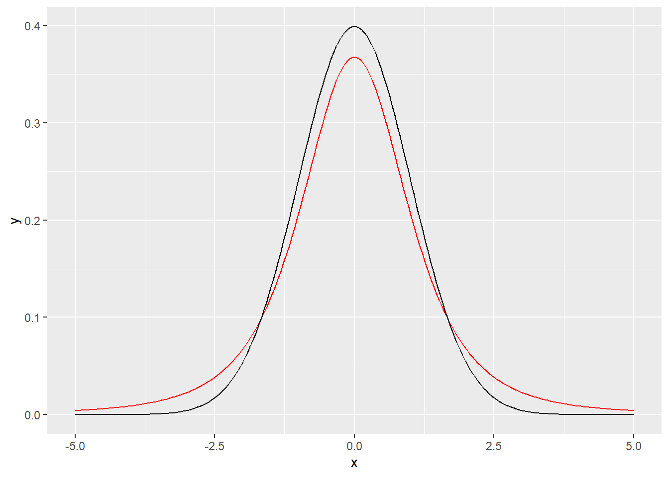

Here the \(t\) distribution is drawn in red (or gray depending on your settings), and the standard Normal is drawn in black for comparison. Notice how the \(t\) distribution has what’s called heavier tails – there’s more probability of getting values far from 0.

There’s actually a whole family of \(t\) distributions, defined by their degrees of freedom (or “df”). Degrees of freedom is a story for another time, but what you should know right now is that the more degrees of freedom a \(t\) has, the “better behaved” it is – fewer extreme values. A \(t\) distribution with infinity degrees of freedom is just a Normal! Actually, infinity starts around 30 – a \(t_{30}\) is effectively the same as a Normal for most purposes.

Here are the \(t\) distributions with 2, 5, and 20 df, plus the Normal:

data.frame(x = c(-5, 5)) %>%
  ggplot(aes(x)) +
  stat_function(fun = dt, n=202, args = list(df = 2),
                color = "orange") +
  stat_function(fun = dt, n=202, args = list(df = 5),
                color = "magenta") +
  stat_function(fun = dt, n=202, args = list(df = 20),
                color = "blue") +
  stat_function(fun = dnorm, n=202, args = list(mean = 0, sd = 1),
                color = "black") +
  annotate("text", x = -3.3, y = .3, label = "t_2, 5, 20, & infinity")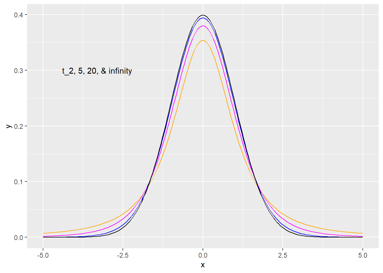

We’ll see the \(t\) distribution pop up a lot – particularly when we are using a sample standard deviation in place of a population standard deviation. Do not be alarmed: you can get probabilities and quantiles and whatnot out of it just like you can with a Normal. It’s just a way of mathematically compensating for the fact that \(s\) is not a perfect estimate of \(\sigma\).