4.2 Inference framework I: hypothesis testing

4.2.1 Introduction

There’s a lot in here, so feel free to take it in chunks! I am assuming you’ve seen this content before, but it may have been a while, and not everyone approaches it exactly the same way.

One reminder before we start: what I’m about to describe is called frequentist inference. This is not the only approach to inference, either mathematically or philosophically. But it is very widely used, so it’s important to understand it. If you’re interested in other approaches to inference, I recommend picking up an elective on Bayesian statistics!

4.2.2 Frequentist inference: the big picture

In general, the goal of inference is to infer something based on what you can observe. In particular, we suppose that there is some population you are interested in, and a particular parameter that describes the behavior of this population. For example, you might be interested in blood pressure. Your population is, let’s say, all US adults, and the parameter you’re interested in is the mean blood pressure, \(\mu\).

You can never observe the whole population, so you can never know the true value of the parameter. But you can guess, or infer, something about it if you take a sample of people and measure their blood pressure. You could calculate a sample statistic from your sample, like, say, the sample mean \(\bar{y}\), and use this to estimate the population parameter.

Frequentist inference takes a particular approach to this. In this philosophy, there is a true, fixed value of the population parameter. It is written on a secret mountain somewhere. It’s something. But you won’t ever know what it is.

What you do know, or at least assume you know, is the probabilistic relationship between that parameter and what you see in your sample. You use this relationship to work backwards from what you see to what you think about the true parameter.

There are two main inference tools or outcomes that you have perhaps encountered: the hypothesis test and the confidence interval.

A hypothesis test says: “Listen, if the true population parameter were some value \(X_0\), would it be pretty normal to see a sample value like this one I have here? Or would this sample value be really unlikely?”

A confidence interval says: “Here’s the whole range of parameter values that would make my sample value reasonably likely.”

4.2.3 The inference framework

So how do you find these things? Well, there’s a procedural framework. This same framework applies no matter what kind of parameter you’re interested in – a mean, a proportion, a regression slope, whatever. It looks like this:

Formulate question
Obtain data
Check conditions
Find the test statistic, and its sampling distribution under H0
Compare observed test statistic to null distribution
Create confidence interval
Report and interpret

Let’s go through in order. For example purposes, let’s say that our variable of interest is blood pressure, and the population parameter we’re interested in is the mean, \(\mu\).

Formulate question:

Start by identifying the parameter, and the corresponding sample statistic. We’re interested in the population mean \(\mu\), so we’ll use the sample mean \(\bar{y}\): the mean of the blood pressure measurements in our sample.

Next, determine the null hypothesis, \(H_0\), and the alternative hypothesis, \(H_A\). The null hypothesis is a statement about the population parameter, which may or may not be true. The null should be two things: boring and tractable. Boring, because you will never be able to confirm it, only reject it or say nothing about it – so rejecting it should be interesting! And tractable, in the sense that you should know how the world works if that null hypothesis were true.

Let’s say my null hypothesis is \(H_0: \mu = 120\). The two-sided alternative would be \(H_A: \mu \neq 120\). Beware – I will never be able to demonstrate that \(\mu\) really is 120! I can only, maybe, find evidence that it isn’t. Otherwise I say nothing about it. So I’d better find it interesting if \(\mu\) is not 120.

Before I go any further, I need to decide on a confidence level, or alpha. How confident do I need to be in my answer? This is one of those “talk to your client” moments. In an exploratory setting, you might be pretty relaxed about this – maybe 95% confidence is good enough. But when the stakes are higher, maybe you need 99% or 99.9% or more. For this example, let’s say \(\alpha = 0.01\), corresponding to a 99% confidence level.

I say you need to decide your alpha first not for mathematical reasons, but for scientific ones. If you don’t start with an alpha in mind, there is a great temptation to wait until you have results, and then pick the alpha that makes them significant. Very sketchy, do not recommend. You may decide in advance to report multiple alphas – you’ll often see this in scientific papers – but your alpha decision should be based on the context of your research problem, not on making yourself look good.

Obtain data:

Next step: get some data! This is a really critical step, and it requires real-world thinking just as much as math or technical knowledge. You need to make sure your sample is representative of your population of interest, and that your variables actually measure the thing you want to measure. You can do all the stats you want, but you can’t compensate for having bad data to start with. If I measure blood pressure only on, say, the members of the varsity meditation team (let’s pretend that’s a thing), I cannot possibly generalize my results to the US population in general.

Properly designing a study or an experiment requires that you’ve already thought about the question – the population of interest, the parameter of interest, the interesting and uninteresting hypotheses, the necessary level of confidence.

Check conditions:

There are some “distribution-free” and “nonparametric” tests that rely on fewer conditions. Bootstrapping is in this category, along with some other things. Most of them are, alas, beyond the scope of this course, but keep an eye out for a possible Stat elective later in life!

Most inference tests rely on certain assumptions and conditions. You may recall phrases like “nearly normal condition” or “constant variance” or “large enough sample.” Which test you’re doing determines which conditions you care about.

For a mean, we generally care about the condition of Normality. That is: do the individual data points come from a roughly Normal distribution? And if they don’t, is our sample size large enough that the Central Limit Theorem will kick in and save us?

Let’s check it for blood pressure. I’m pulling a sample of 250 people from the NHANES public health study.

library(NHANES)
set.seed(2) # force R to take the same "random" sample every time the code runs!
sam_NHANES = NHANES %>%
  filter(!is.na(BPSysAve)) %>% # only include people who *have* BP measurements
  slice_sample(n = 250, replace = FALSE)

Let’s check a histogram of systolic blood pressure:

sam_NHANES %>%
  ggplot() +
  geom_histogram(aes(x = BPSysAve), bins = 20)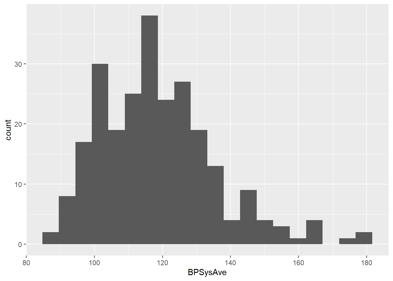

Mmm. Not super normal, really. Recall the “shape, center, and spread” catchphrase for describing distributions. The shape of this distribution is not very symmetric, like a Normal would be; instead it’s skewed right.

To confirm, we could try a Normal probability plot or QQ plot. If you haven’t met these before, basically, they compare the quantiles from my sample to the quantiles of a Normal distribution. If my sample values follow a Normal distribution, the points will more or less fall along a straight line.

sam_NHANES %>%
  ggplot(aes(sample = BPSysAve)) + # specifying aes() here means *all* the later commands will use it
  stat_qq() +
  stat_qq_line()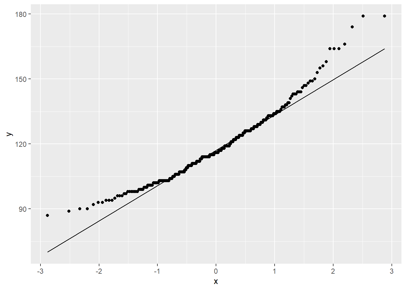

Again, not so great. QQ plots always look a bit funky out at the tails, but a big curve like this is a definite indication of non-Normality.

You may recall that one way of dealing with this is to try a transformation on the data. We’ll see this again in the future, but for now, I’ll try taking the log of the values:

sam_NHANES = sam_NHANES %>% mutate("logBPSysAve" = log(BPSysAve))

sam_NHANES %>%
  ggplot() +
  geom_histogram(aes(x = logBPSysAve), bins = 20)

sam_NHANES %>%
  ggplot(aes(sample = logBPSysAve)) +
  stat_qq() +
  stat_qq_line()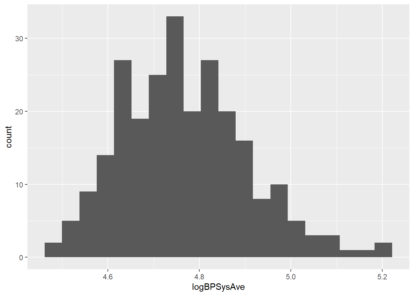

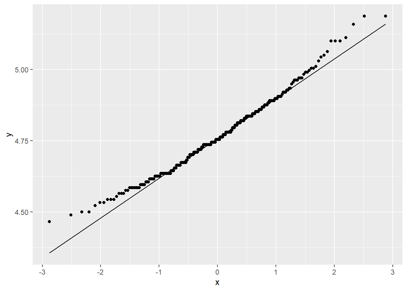
Well, not perfect, but better. Probably good enough; with a sample size of 250, my analysis should be pretty robust to non-Normality.

I don’t see any other concerning behavior, like extreme outliers, multiple modes, or weird gaps, so I’d say we’re good on the nearly-Normal side of things.

There’s one assumption that you may remember cropping up in all the inference tests, no matter what parameter you were investigating: independent observations. Since we’re working with observational data, we want to know that we got a nice, random, unbiased sample – we didn’t, say, sample a bunch of people from the same family or something. We’ll have to trust the NHANES study designers on that, so on we go!

Find the test statistic, and its sampling distribution under \(H_0\)

A statistic is any value you calculate from your data, and a test statistic is a statistic you calculate to help you do a test.

For a mean, the test statistic is the \(t\) statistic. You start with the sample mean \(\bar{y}\), then standardize it: \[ t = \frac{\bar{y} - \mu_0}{s/\sqrt{n}} \]

Here, \(\mu_0\) is the null value of the parameter – in our example, \(H_0\) was that the true average blood pressure was 120. But remember, we took a log! If the average blood pressure is 120, the average log blood pressure is \(\log(120)\). So our \(\mu_0\) is \(\log(120)\), which is about 4.8. That \(s\) in the denominator is the sample standard deviation. Using \(s\) here instead of \(\sigma\), the true population SD, is why this is a \(t\) statistic and not a Normal, or \(z\), statistic!

Let’s find this for our sample:

sam_ybar = sam_NHANES$logBPSysAve %>% mean(na.rm = TRUE) # remove NAs
sam_s = sam_NHANES$logBPSysAve %>% sd(na.rm = TRUE)
sam_t = (sam_ybar - log(120)) / (sam_s/sqrt(250))
sam_t

## [1] -2.42752

Meanwhile, we also happen to know that if the null hypothesis is true, this \(t\) statistic follows a Student’s \(t\) distribution with \(n-1\) degrees of freedom. That means that if \(H_0\) were true, and we took a whole bunch of samples and did this calculation for each one of them, and then made a histogram of the distribution of all those individual \(t\)’s, it would look like this:

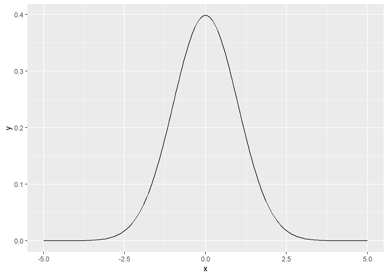
That’s its null sampling distribution, or its sampling distribution under \(H_0\). Different test statistics have different null sampling distributions.

Compare observed test statistic to null distribution

Well, we have this picture of what \(t\) statistics tend to look like if \(H_0\) is true. We also have an actual \(t\) statistic that we calculated from our observed data. Let’s compare:

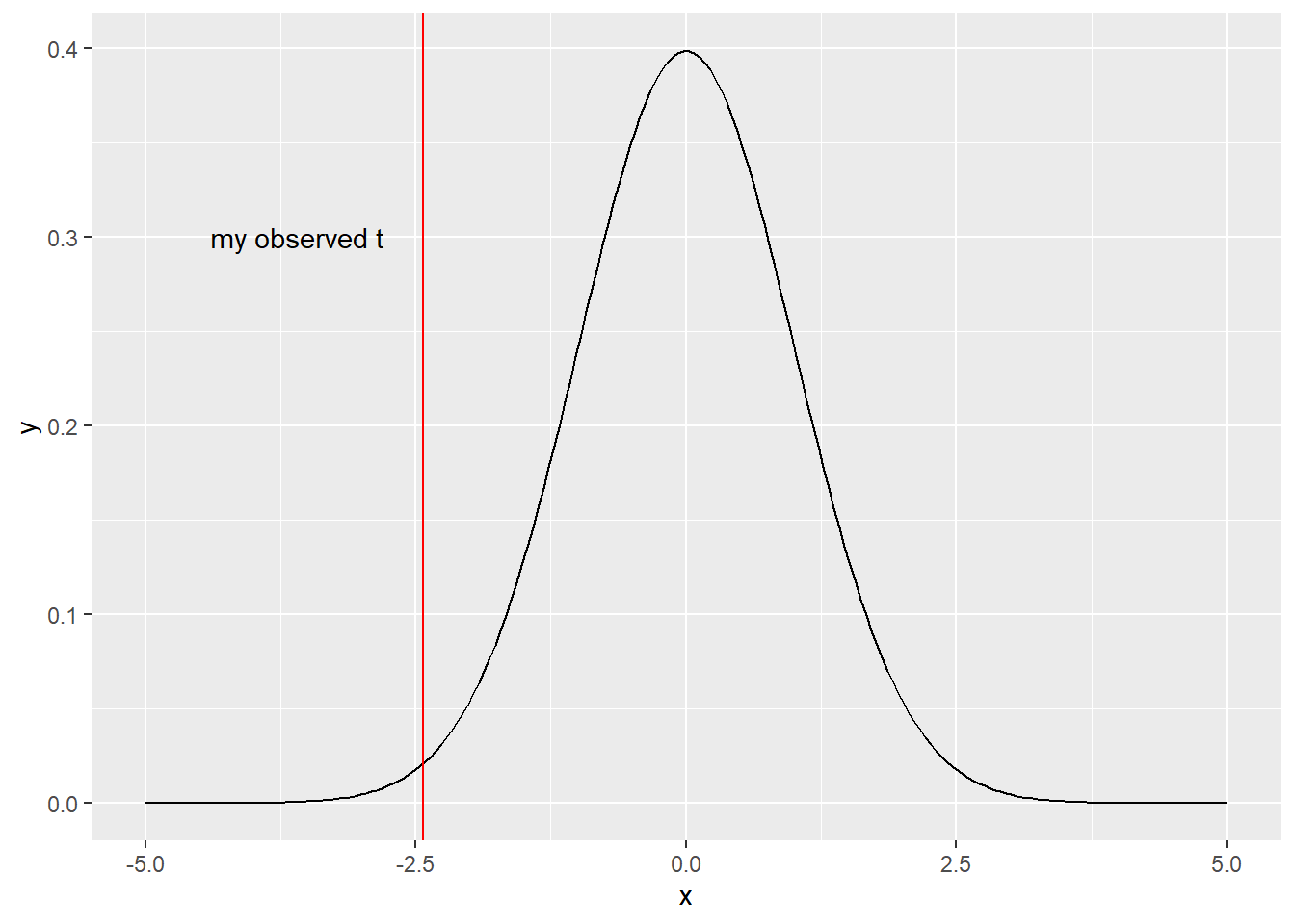
Huh. That seems…questionable. If I were drawing values from this null distribution, I’d be somewhat unlikely to draw something so far out there. Or as the statisticians phrase it: to get a value as or more extreme – where “extreme” means far from the center of the distribution.

Suppose I decided that, yes indeed, that value is unlikely. One might even say weird. Now, as a statistician, I think that weird things happen, but not to me. Then I’d conclude that since this value would be weird if \(H_0\) were true, and weird things don’t happen to me, well, \(H_0\) must not be true after all.

But, I don’t know, maybe it’s not that unlikely. How weird is weird, anyway? We quantify this idea with a p-value. A p-value is a probability: specifically, it’s the probability of observing a value at least this extreme, if the null hypothesis is true. P-values have, like, a lot of problems, but again, they’re really common so it’s good to remember where they come from.

I can actually get the p-value semi-manually by finding the tail probabilities of the \(t\) distribution:

p_val = 2*(pt(sam_t, df = 250-1, lower.tail = TRUE))
p_val

## [1] 0.01591225

If \(H_0\) really is true, I’d have a 1.5% chance of getting a test statistic at least this far from 0.

Then I compare that to the alpha I decided on way back at the beginning, 0.01. And I conclude: meh. To me, something that happens 1.5% of the time doesn’t count as weird, so it’s still plausible to me that \(H_0\) is in fact true. Or, to put it technically: because my p-value is higher than my alpha, I fail to reject \(H_0\). Note that I don’t accept \(H_0\)! I’m not saying that \(H_0\) is true. I just haven’t found sufficiently strong evidence against it.

Note that if my p-value were lower than alpha, I would reject \(H_0\). In fact, I’d do that if I’d set \(\alpha = 0.05\). But I decided at the beginning that I needed to be more confident than that! I refuse to get all excited unless I see stronger evidence against \(H_0\).

Response moment: When I calculated my p-value, I used pt to get a probability, and then multiplied it by 2. Why did I do this doubling?