10.2 Influential points: IRLS robust regression
This idea we had of weighting different observations is pretty clever! There are lots of other ways we might choose to assign weights to different points, depending on our goals or what we think the issues are with the dataset. Here, we’ll look at weighting as a way of handling yet another regression-conditions problem: influential points.
We call this procedure robust regression. In statistics, “robust” often refers to a method that isn’t strongly influenced by outliers or special points.
10.2.1 Influential points
You’re used to looking for outliers or special points on leverage/residual/Cook’s-distance plots. In particular, you might worry if you see points with high leverage and a large residual (or large Cook’s distance, which combines both of those things). But what do you do with them if you see them?
Well, you can drop ’em entirely if you have a good reason. But what if you don’t? Can we express “I’d rather not have this particular point running the show” without just deleting it from the dataset?
Sure you can! With the magic of weighted least squares.
Let’s use some synthetic data for an example:
set.seed(1)
x = runif(100,0,10)
y = 5 + 2*x + rnorm(100,sd=5)
x = c(x,20)
y = c(y, 4)
influ.dat = data.frame(x,y)
ggplot(influ.dat) +
  geom_point(aes(x=x, y=y))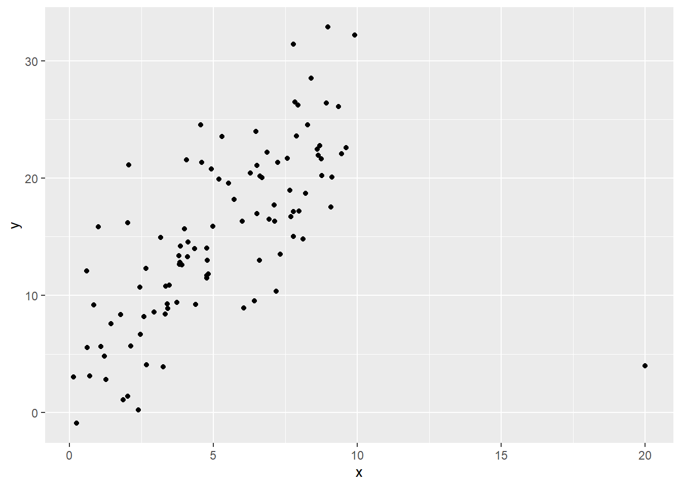
Fig. 1: yikes
So we’ve got this one point that is super influential – we want it not to have such a big impact on the coefficient estimates.
10.2.2 The robust regression procedure
Let’s give each point its very own weight \(w_i\) in the regression, where it gets less weight if its residual is especially large in magnitude. Notice that in the IRLS procedure for non-constant variance we assumed there was a linear relationship between a point’s predictor values and its error variance, and thus its weight. But now, we do not assume that the weights are a function of a predictor or anything; we’ll just determine them individually for each point, based on that point’s residual.
The procedure is similar, though!
In the non-constant variance version, we just used the reciprocal: \(w_i = 1/\hat{s}_i\). That meant that points with larger estimated variance/SD got smaller weights.
We could define a similar weight function here, as \(w(u) = 1/|u|\). But that’s a pretty straightforward relationship, and may not work so well for individual residuals. (For one thing, what if you have a residual of 0?) So we usually use a function that has a more complicated equation but is better behaved.
Step 1: Choose a weight function to define the relationship between a point’s residual and the weight it gets. We want larger residuals (either positive or negative!) to be associated with smaller weights…but there are a lot of ways to do that.
For example, you could use the bisquare weight function, shown here as a function of some value \(u\):
\[w(u) = \begin{cases} [ 1 - \left(\frac{u}{4.685}\right)^2]^2\text{ where }|u|<4.685 \\ 0 \text{ where }|u|>4.685\end{cases}\]
u = seq(-4.685,4.685,by=.1)
plot(u,(1-(u/4.685)^2)^2,type='l',ylab='Weight Function')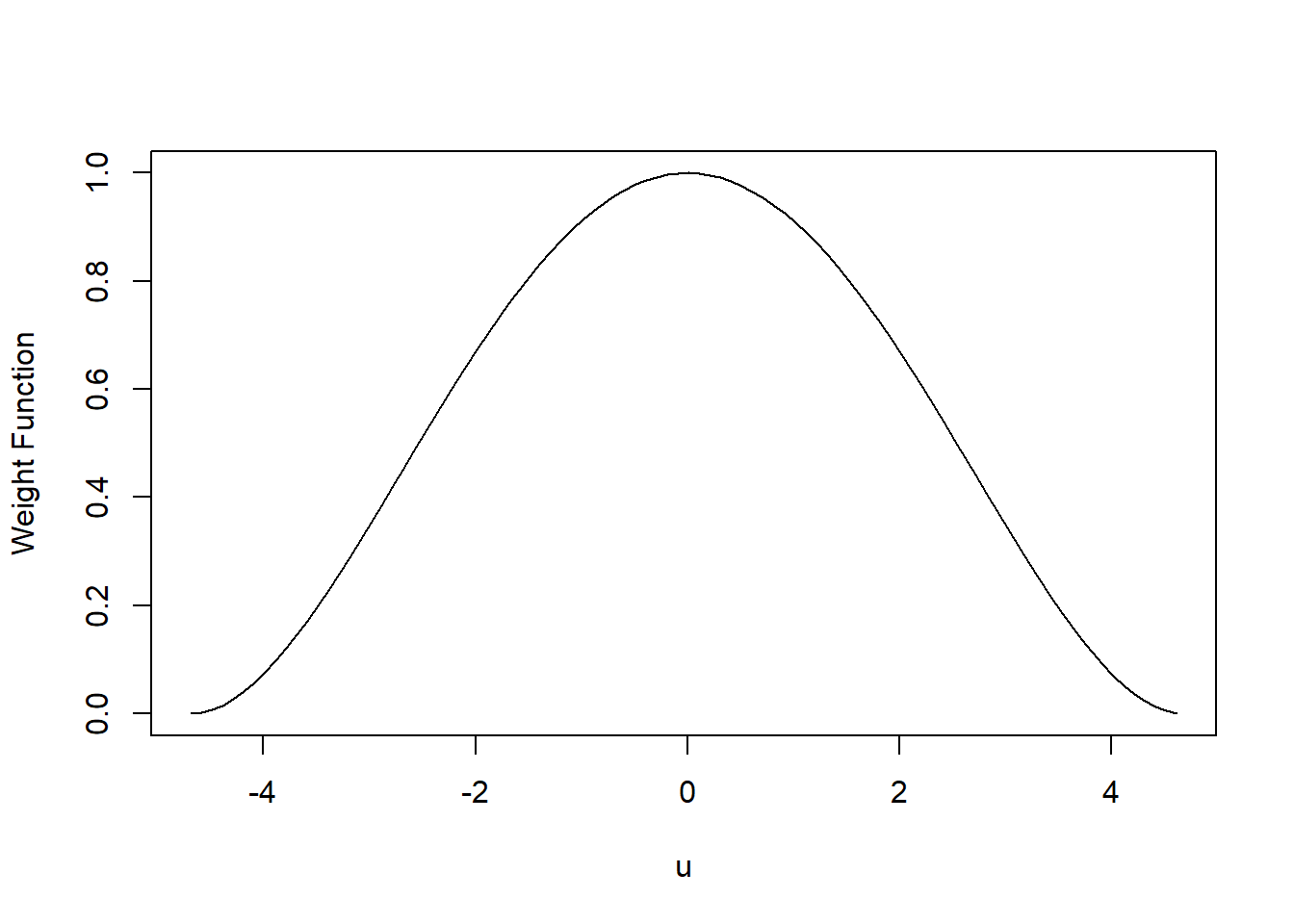
This is a weird function and we won’t talk about where it comes from, but do note that 4.685 is chosen to make this procedure efficient for data that come from a normal regression model. So it’s good to check those residuals for normality before using this!
Efficient, if you’re wondering, means that this procedure provides the best possible performance given the sample size you have. Statistical efficiency is a topic for a more theoretical class, but now at least you’ve seen the term :)
Values of \(u\) near 0 get larger \(w(u)\) (aka weight) values, and the weights get lower for values of \(u\) farther from 0.
Step 2: Initialize weights for each point (you could make them all equal to start; that’s equivalent to ordinary least squares).
Step 3: Do weighted least squares (using these initial weights), and find the fitted model, according to the weighted normal equations:
\[\boldsymbol b_{w} = (\boldsymbol X' \boldsymbol W \boldsymbol X)^{-1}\boldsymbol X' \boldsymbol W \boldsymbol y\]
Use this model to get an initial set of residuals \(e_i\).
Step 4: Use the residuals from step 3 to get a new set of weights.
The conventional procedure for this has two parts. First, for each point, scale the residual by calculating
\[u_i = \frac{e_i}{MAD}\]
where
“MAD” stands for “median absolute difference,” which you will see is exactly what this is based on. It’s a way of expressing the spread (and thus the scale) of the residuals, although not one of the ways you’re used to! Scaling by this factor just ensures that your results don’t depend on the units of your response variable.
Again, we won’t derive this, but it’s a fun fact that 0.6745 provides an unbiased estimate of \(\sigma\) for independent values from a normal distribution.
\[MAD = \frac{1}{.6745}median(|e_i - median(e_i)|)\]
Then plug these \(u_i\) into your chosen weight function (like the bisquare above) to obtain \(w_i\) for each point, and thus a new weight matrix.
Step 5: Repeat steps 3 and 4: new weights give you new coefficient estimates, which give you new residuals, which give you new weights, and so on. Keep going until the coefficients stabilize – that is, until they don’t change much from one iteration to the next. As usual, R has its own idea of when to stop.
Here’s what this looks like in R. First we have the fitted coefficients from ordinary least squares, where we don’t take into account that that one point is influential; then we have the fitted coefficients from robust regression.
lm(y~x, data=influ.dat)$coef## (Intercept) x
## 7.321942 1.471400require(robustreg)
robustRegBS(y~x,data=influ.dat)$coef##
## Robust Regression with Bisquare Function
## Convergence achieved after: 10 iterations## (Intercept) x
## 3.635919 2.197912That influential point sure dragged down the slope in the original version! But by downweighting it, we were able to see that a steeper slope was better overall.