1.8 Goodness of Fit (SLR Edition)
1.8.1 The missing piece
Recall the usual list for describing the relationship between two quantitative variables: direction, form, and strength. We’ve now seen a number of tools that can help describe those characteristics. It’s important to note, though, that both correlation and linear regression assume a particular form – a straight-line relationship. These tools can’t actually tell us if there is some curved or nonlinear relationship between the variables. This is one of many reasons why it’s important to plot your data!
Assuming that we have a linear relationship, correlation can tell us about the direction of that relationship – based on its sign – and also something about the strength of the relationship – based on whether it’s close to \(\pm 1\).
Fitting a regression line also tells us about the direction of the relationship. It does better than that, in fact: it tells us what the line actually is: its y-intercept and, more interestingly, its slope.
But you may notice that the regression line doesn’t tell us about strength.
Let’s look at two different example datasets. These are simulated data points – I’ll tell you how I simulated them later.
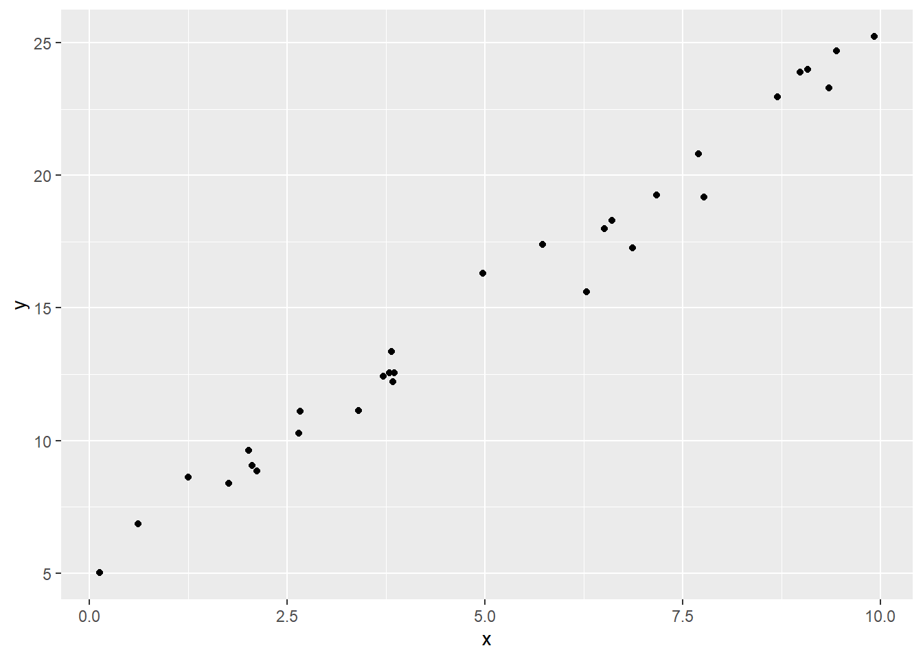
Here’s a dataset that shows a strong, positive linear relationship between \(x\) and \(y\):
And here’s one that shows a somewhat weaker positive linear relationship:
weak_dat = data.frame("x" = x_vals,
                        "err" = rnorm(30, sd = 5)) %>%
  # rowwise() %>%
  mutate("y" = c_intercept + c_slope*x + err) %>%
  ungroup()
weak_dat %>%
  ggplot() +
  geom_point(aes(x = x, y = y))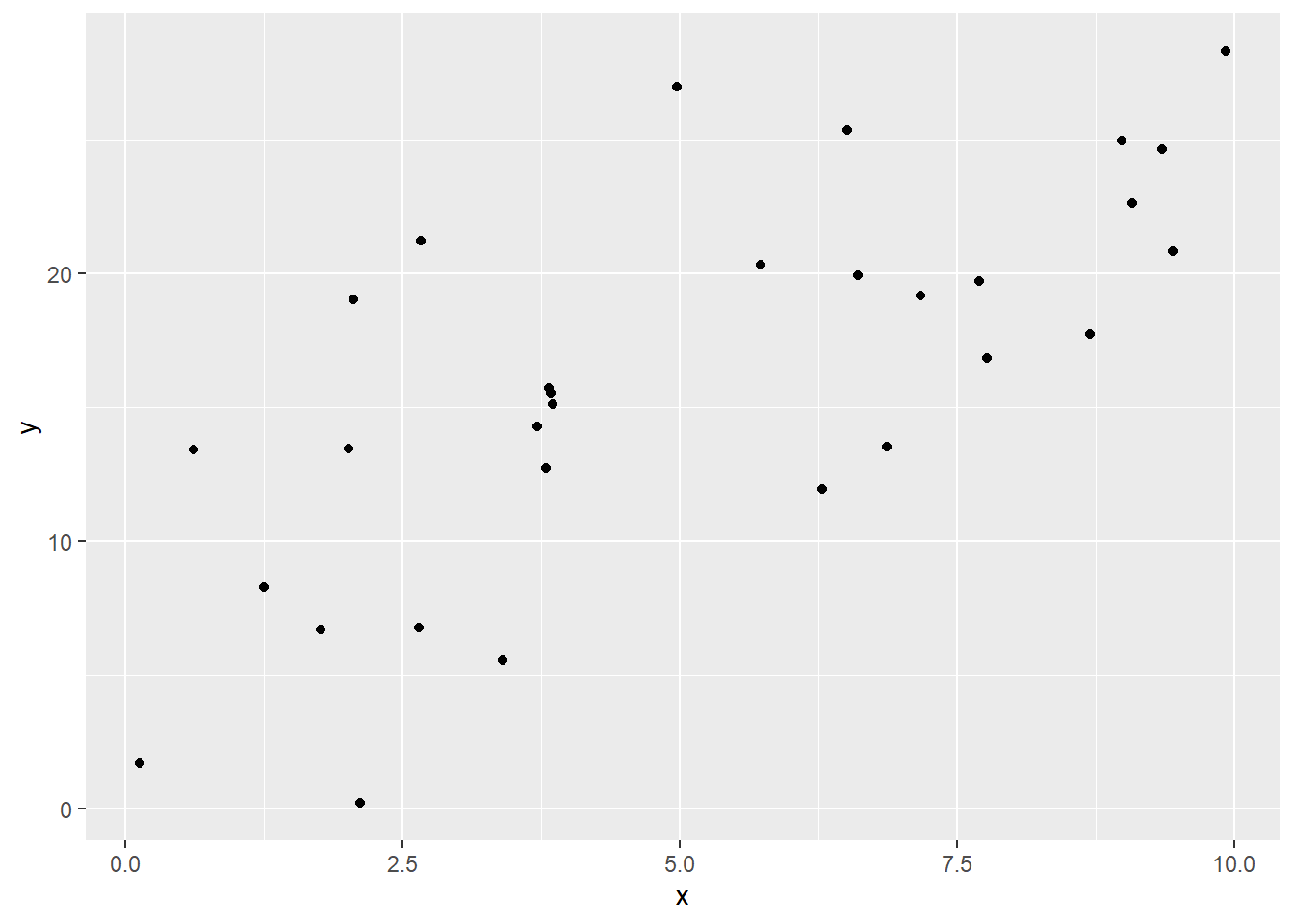
Visually, we can talk about the difference between these two datasets as one of them being more “spread out,” or one of them having points more “tightly along a line.” This reflects what we call the goodness of fit of the line. So how can we quantify this rather than just eyeballing it?
1.8.2 The spread of the residuals
If we want to talk about how well the line does, or how closely the points fit the line, then maybe it makes sense to look at the residuals – how far the points are from the line. In a really spread-out dataset with only a vague trend, even if we use the best-fit line, we’ll still have sizeable residuals; but in a dataset where the points stay really close to the line, the residuals will be small.
So…perhaps we could find the average residual?
strong_lm = lm(y ~ x, data = strong_dat)
weak_lm = lm(y ~ x, data = weak_dat)

strong_lm$residuals %>% mean()
## [1] 1.525111e-17weak_lm$residuals %>% mean()## [1] 1.998691e-16Welp. Those values are both “machine 0” – as close to 0 as R can get given the limits of my computer’s calculation.
Turns out, the mean of the residuals is always 0, no matter whether the linear fit is weak or strong. They just cancel each other out: some residuals are positive, and some are negative.
What we really want to know is how far from 0 the residuals tend to be – that is, their spread. So instead of the mean, we might be interested in the variance or the standard deviation of the residuals. For exciting mathematical reasons that we won’t go into here, we use what’s called the standard error of the residuals, which involves dividing by \(n-2\) instead of \(n-1\):
\[s_e = \sqrt{\frac{\sum_i{e_i^2}}{n-2}}\] Conveniently, R actually calculates this for us while fitting the linear model. We can acces it like this:
summary(strong_lm)$sigma## [1] 0.7911047summary(weak_lm)$sigma## [1] 5.207174Now, in and of itself, this value isn’t meaningful, because we need to know what scale we’re talking about.
Fortunately, the standard error of the residuals has the same units as the original \(y\) values. This can come in handy for reality-checking a line’s results. If the residuals are Normally distributed, we can use the 68-95-99.7 rule: 95% of residuals will be within two-ish \(s_e\)’s of 0. That tells us what size residuals we can generally expect – how far off we expect most of our predictions to be. Now, we can (and will) get much more specific about how good we think our prediction is for a particular \(x\) value. But this is just a nice way of getting a general sense of how the predictions will do.
The residual standard error also becomes very handy when we compare it to other things, as we’ll see in a moment.
1.8.3 R-squared
Let’s step back for a second. We already have a tool that measures the strength of a linear relationship: the correlation. So we could just look at the correlation, \(r\), between \(x\) and \(y\) in each case:
cor(strong_dat$x, strong_dat$y)## [1] 0.991406cor(weak_dat$x, weak_dat$y)## [1] 0.7080689Both are positive – matching the direction of the relationship – but the correlation in the strong-relationship dataset is considerably closer to 1.
But wait: there’s more! There’s a variation on this that ends up being more useful to interpret. It’s called \(R^2\), and it is, literally, equal to \(r\), the correlation, squared.
cor(strong_dat$x, strong_dat$y)^2## [1] 0.9828858cor(weak_dat$x, weak_dat$y)^2## [1] 0.5013616How is \(R^2\) different from correlation? Well, it’s on a bit of a different scale, for one thing. Since it’s obtained by squaring, it can’t be negative, so it doesn’t reflect the direction of the relationship, only the strength. Its minimum value is 0, indicating no correlation. Its maximum value is 1, although you should worry if you get an \(R^2\) of exactly 1, just like you should if you get a correlation of exactly \(\pm 1\). That never happens in real life, so it probably means something is wrong with your data.
But the other interesting thing about \(R^2\) has to do with regression.
When we fit a regression line of \(y\) on \(x\), our goal is to predict or explain the \(y\) values. All our data points have different \(y\) values – but why? To some extent, it’s just because, hey, life is variable. But to some extent, we can explain those different \(y\) values by looking at the \(x\) values. For example, suppose \(x\) is a child’s age and \(y\) is their height. Well, different children have different heights. But there is a relationship between age and height. So if we see that, say, a particular child is quite tall, we can partly explain that by taking their age into account. Only partly, though! There’s still additional variation in children’s heights on top of that.
What we might like to ask, though, is how much of the variation in height, \(y\), we can account for by looking at age, \(x\), and how much is left over – unexplained by \(x\). If we can account for almost all the variation in height by looking at the children’s ages, then our line – our model, if you will – is doing a good job and making good predictions; the data fit well.
It turns out that \(R^2\) measures this very thing. \(R^2\) is equal to the fraction of the variation in \(y\) that can be explained by the model – that is, by \(x\). And then \(1-R^2\) is the fraction of the variation in \(y\) that can’t be explained using \(x\): the leftover variance, if you will.
For example, in our simulated data, we can calculate the variance of the \(y\) values in each dataset:
strong_y_var = strong_dat$y %>% var()
strong_y_var
## [1] 35.3078weak_y_var = weak_dat$y %>% var()
weak_y_var## [1] 52.50232Now, how much of that variation goes away when we take \(x\) into account? Well…how much of it is left over? That’s just the variance of the residuals.
strong_res_var = strong_lm$residuals %>% var()
strong_res_var
## [1] 0.6042657weak_res_var = weak_lm$residuals %>% var()
weak_res_var## [1] 26.17967So what fraction of the variance in \(y\) is not explained by \(x\) – is left over?
strong_res_var/strong_y_var## [1] 0.01711423weak_res_var/weak_y_var## [1] 0.4986384Finally, let’s subtract these values from 1: that gives us the fraction of the variance in \(y\) that is explained by \(x\).
1 - strong_res_var/strong_y_var## [1] 0.98288581 - weak_res_var/weak_y_var## [1] 0.5013616Those are the \(R^2\) values for each line! In the dataset with the strong relationship and well-fitting line, almost all the variation in \(y\) can be accounted for using \(x\). But in the weak-relationship dataset, using \(x\) only explains about half the variation in \(y\); the rest is left unexplained.
Again, fortunately, we do not have to do this whole calculation out every time. R calculates \(R^2\) for us:
summary(strong_lm)$r.squared## [1] 0.9828858summary(weak_lm)$r.squared## [1] 0.5013616Response moment: What qualifies as a “good” \(R^2\) value?
1.8.4 P.S. (for the curious)
Wondering how I simulated the points in these datasets? I did so by taking some \(x\) values, calculating their \(\widehat{y}\) values using a line, and then adding random errors to get the “actual” \(y\) value for each point. Like this:
set.seed(1) # always simulate responsibly: set your seed
x_vals = runif(30, min = 0, max = 10)
  # (r)andom draws from a (unif)orm distribution
c_intercept = 5
c_slope = 2

strong_dat = data.frame("x" = x_vals,
                        "err" = rnorm(30, sd = 1)) %>%
          # (r)andom draws from a (norm)al distribution
  mutate("y" = c_intercept + c_slope*x + err) %>%
  ungroup()

weak_dat = data.frame("x" = x_vals,
                        "err" = rnorm(30, sd = 5)) %>%
  mutate("y" = c_intercept + c_slope*x + err) %>%
  ungroup()
The difference between strong_dat and weak_dat is that the errors in weak_dat were generated to have a much larger standard deviation! So it makes sense that \(s_e\) was much larger for the weak dataset than the strong one. Of course, \(s_e\) is just an estimate, so it won’t exactly match the “true” error SD that I used. But it’s not too far off.