1.7 SLR: Least Squares

1.7.1 What is a “good” line?

When we do a linear regression, our goal is to draw a line through a bunch of data points, or observations. This line describes what we think is an underlying relationship between the X variable – the predictor – and the Y variable, aka the response.

But, as previously observed, we can’t get a straight line that goes through all the points. We just want to get a line that gets as close to the points, overall, as possible.

In particular, keep in mind that we define a line using its intercept and its slope. So when we say “find the best-fit line,” we mean: “find the values for intercept \(b_0\) and slope \(b_1\) so that, overall, we minimize the distance between the resulting line and the data points.”

1.7.2 Least squares fits

Now, there’s more than one way to talk about “the distance from a point to the line.” But for our purposes, we use what you might call the vertical distance. Like so:

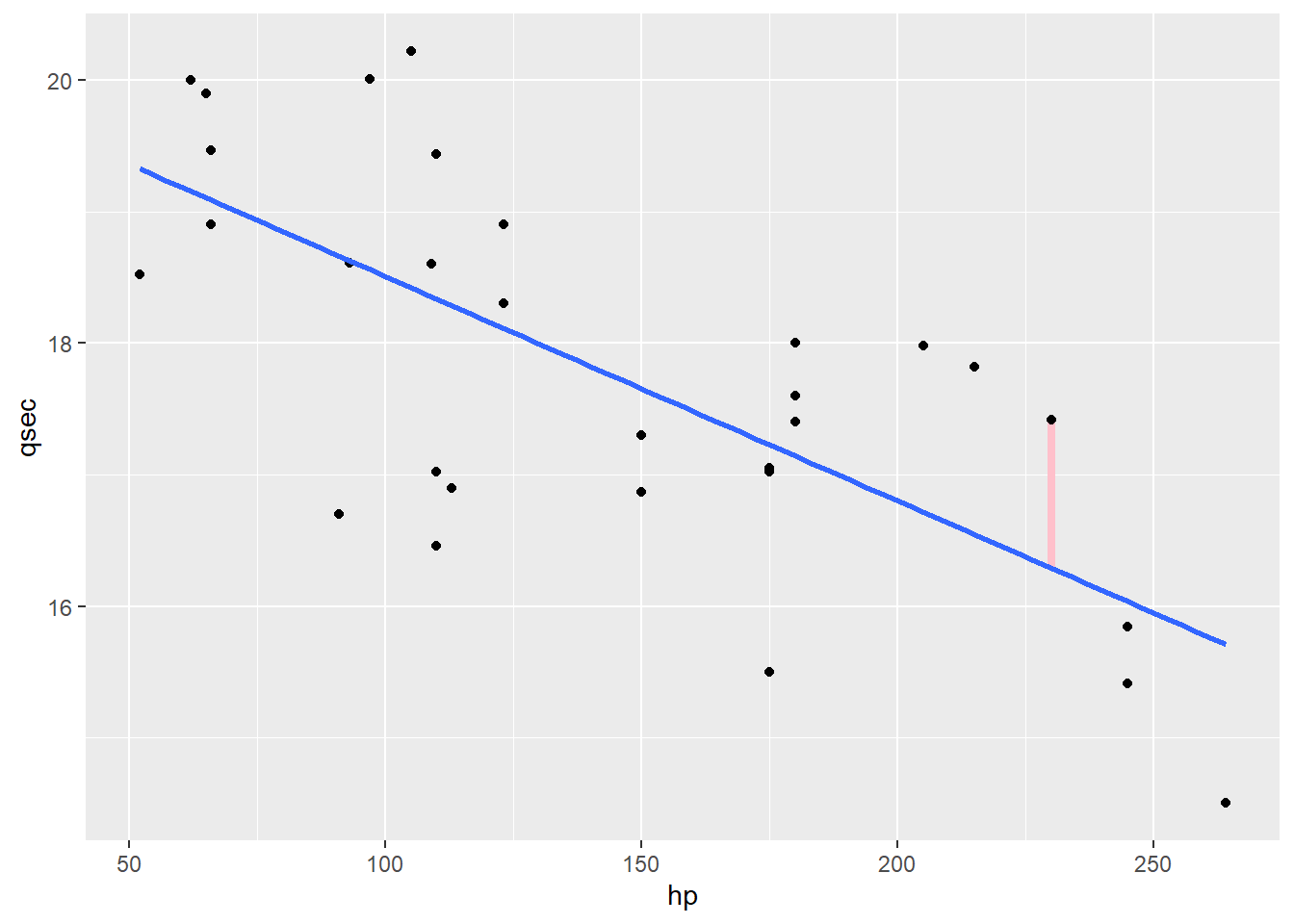
We can find that vertical distance for every point – here’s a few more:

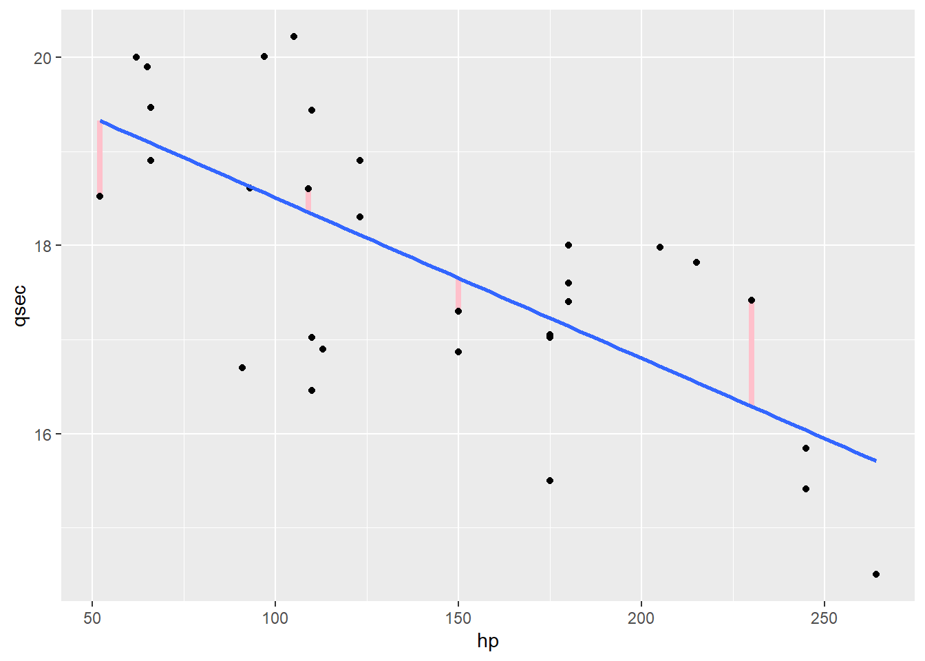
You may recognize these “distances” as the residuals for each point: the true \(y\) value minus the fitted \(y\) value, \(qsec - \widehat{qsec}\). We’d like to find the line that minimizes these distances overall.

But it’s not enough just to minimize the sum of the residuals. Why?

Response moment: Why can’t we just work with the sum of the residuals?

In order to deal with this problem, we first square each residual before summing them up, yielding the sum of squared residuals. Then we find the slope and intercept values that minimize this sum of squares.

Now, we can do this with a little light multivariable calculus, but happily, there is a closed-form solution – a simple formula for the optimal choices of \(b_1\) (slope) and \(b_0\) (intercept). It is thus:

\[b_1 = r \frac{s_y}{s_x}\] and

\[b_0 = \overline{y} - b_1 \overline{x}\]

1.7.3 Slope and correlation

Let’s look at that formula for the slope:

\[b_1 = r \frac{s_y}{s_x}\]

What are these pieces?

Well, \(r\) is just the correlation between \(x\) and \(y\). And \(s_y\) and \(s_x\) are the standard deviations of the \(y\) values and \(x\) values of all the points, respectively.

So what this tells us is that the regression slope is a scaled version of the correlation. This explains why the sign of the regression slope and the sign of the correlation always agree, but the slope can be any number, while the correlation is stuck between -1 and 1.

The fact that \(s_x\) and \(s_y\) are in here also tells you something about how the regression slope will react to transformations of \(x\) and \(y\). Remember, standard deviation – a measure of spread – doesn’t care about where the center is. So if you shift \(x\) or \(y\), it won’t matter. But if you scale \(x\) or \(y\), that will change the standard deviation – so the regression slope will change. Of course, you’d need to account for this scaling when you were interpreting the regression slope!

1.7.4 An important point (literally)

I said before that the intercept wasn’t always very interesting in context, which is true. But it is necessary mathematically, and its formula can also show us something interesting. Here it is:

\[b_0 = \overline{y} - b_1 \overline{x}\]

Let’s rearrange it a bit:

\[\overline{y} - b_1\overline{x} = b_0\] \[\overline{y} = b_0 + b_1\overline{x}\]

Now compare the regression equation:

\[\hat{y} = b_0 + b_1 x\]

So what the intercept equation tells us is: if we plug in \(\overline{x}\), the mean value of the predictor, then our predicted response is…the average value of the response. Which makes sense, on some level. A data point with an average value of \(x\) could be expected to have an average value of \(y\).

So in some sense, the intercept is the value that makes the line pass through the point \((\overline{x}, \overline{y})\). This also tells us something about how that line behaves when we transform the variables. Any transformation that changes \(\overline{x}\) or \(\overline{y}\) is going to change the intercept, including shifting and scaling.