1.11 Inference for a Regression Slope
1.11.1 Return of the inference framework
Remember this thing? We’ve seen it before, doing inference on means.
- Formulate question
- Obtain data
- Check conditions
- Find the test statistic, and its sampling distribution under H0
- Compare observed test statistic to null distribution
- Create confidence interval
- Report and interpret
We’re now going to use this same framework to do inference on the slope in a linear regression. Basically, we’ll be interested in finding out whether we’re really confident that there truly is a relationship between \(x\) and \(y\).
1.11.2 Some notation
Back in the day, when we were working with means, we used different notation to refer to the parameter – the true population value, which we could never observe – as opposed to the sample statistic, which we calculated from our sample and used as an estimate of the parameter. The parameter was \(\mu\), and the corresponding sample statistic was \(\overline{y}\).
We’ll do something similar here. As before, we’ll use Greek for the parameter/population/True version:
\[y = \beta_0 + \beta_1 x + \varepsilon\]
But for the version where we calculate things based on our sample, we’ll use Roman lettering:
\[y = b_0 + b_1 x + e\]
Now \(x\) and \(y\) are the same in both these versions; \(x\) is the point’s predictor value, and \(y\) is the value of the point’s response. But the coefficients are different. The parameter version describes the True Line – the line we would fit if we had all the data points in the whole population. The sample version describes the best-fit line created using our sample dataset. So \(b_0\), the intercept of our fitted regression line, is an estimate of \(\beta_0\), the true intercept. And, more usefully, \(b_1\), the slope of our fitted regression line, is an estimate of \(\beta_1\), the true slope.
Let’s explore an example. Suppose we’re interested in using people’s age to predict their systolic blood pressure. We take a sample of 50 folks from the NHANES public health study, but our population of interest is, say, all US residents.
set.seed(12) # sample responsibly
bp_dat = NHANES %>%
  filter(!is.na(BPSysAve)) %>%
  slice_sample(n = 50)
If we could actually observe the entire population, our regression equation would be:
\[BP = \beta_0 + \beta_1 Age + \varepsilon\]
Notice that there’s still an error term here, \(\varepsilon\). Even if we had the entire population, and could find the best possible line, we still wouldn’t be able to predict every person’s blood pressure exactly right using their age. People of the same age can have lots of different blood pressures. So when we predict someone’s blood pressure we will have error, even if we are using the True Line.
Now of course we don’t have the entire population, so we can’t actually fit this line; so we’ll never know exactly what those \(\beta\)’s, the true intercept and slope, are. We just have 50 people.
bp_dat %>%
  ggplot() +
  geom_point(aes(x = Age, y = BPSysAve))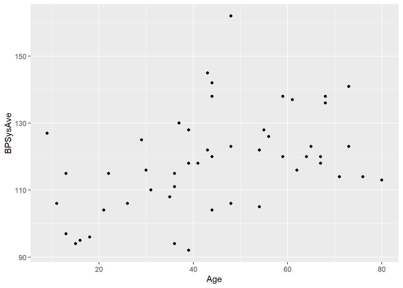
When we fit a regression line using this data, we’ll get the fitted or estimated regression equation:
\[BP = b_0 + b_1 Age + e\]
We can use R to find the \(b_0\) and \(b_1\) values based on our sample:
bp_lm = lm(BPSysAve ~ Age, data = bp_dat)
bp_lm$coefficients
## (Intercept) Age
## 103.8526796 0.3324511So our fitted regression line is:
\[BP = 103.9 + 0.332 Age + e\]
The \(e\) here is the residual for that point. It’s equal to the difference between that person’s actual blood pressure and what we’d predict based on their age: \(BP- \widehat{BP}\).
When we do inference with regression, our goal is to use the estimated coefficients – okay, mostly just the estimated slope coefficient – to make guesses about what the true coefficient actually is.
1.11.3 Hypotheses
So what would be the null hypothesis here? Remember that \(H_0\) is supposed to be the “boring scenario.” Well, a regression is boring when…it doesn’t help. If there is no actual (linear) relationship between age and blood pressure, then age isn’t a useful predictor and we might as well just go home.
Mathematically, what would this mean? Well, if age isn’t associated with higher blood pressure or lower blood pressure, then the slope coefficient of age would be…zero. No matter how old you are, I’ll predict the same thing for your blood pressure.
Formally, this would be:
\[H_0: \beta_1 = 0\]
It is possible to use other null hypotheses, but quite rare. You’d need a really good reason based on the problem context.
What about the alternative? The vast majority of the time, we use a two-sided alternative for regression tests:
\[H_A: \beta_1 \ne 0\]
You could have a situation where you’re only interested if the slope is positive, or only interested if it’s negative. But most often you’re interested if there is a slope at all – if \(x\) and \(y\) have some kind of relationship, in either direction.
The next thing to do in the inference framework is to gather some sample data (if someone hasn’t handed it to you already). Remember that this is the step to think about when you’re considering the independence assumption! You want to be sure your sample is representative of the population, unbiased, and random so that there’s no relationship between different data points. Don’t go measure the blood pressure of a bunch of people in the same family, or a bunch of athletes, or whatever.
1.11.4 Check conditions
Assuming that the independence condition is met – and the people who did the NHANES study were professionals so I’m going to roll with it – let’s check the others with some plots.
Here’s the plot of residuals versus fitted values:
bp_lm %>% plot(which = 1)
From this I can see that the spread of the residuals is about the same all the way across, so I feel good about the equal variance condition. I don’t see any real bends here either, so we’re probably okay on linearity. There does seem to be a potential high outlier (person no. 28), but since I can’t go find out who that person was and what their deal was, and it’s not suuuper extreme, I’m going to leave them in for now.
Now let’s try the Normal QQ plot of residuals:
bp_lm %>% plot(which = 2)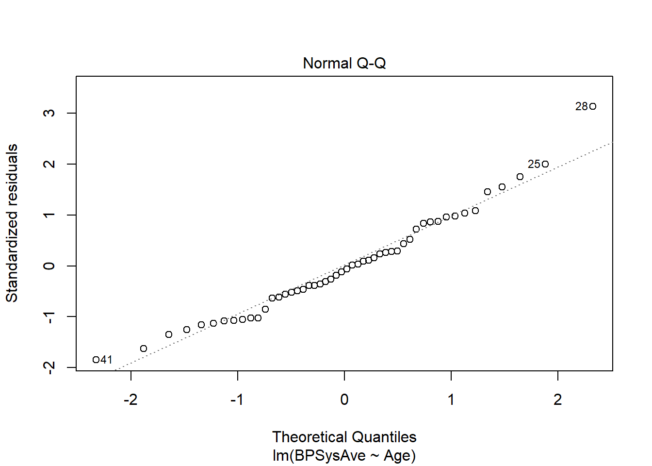
Looks pretty straight along the line, except for good old point #28. So Normality seems to be satisfied. Onward!
1.11.5 Test stat and sampling distribution
Back in the day, when we wanted to do inference on the mean \(\mu\), we took our sample statistic \(\overline{y}\) and standardized it by dividing by its standard error. This gave us a \(t\) statistic, which we could then compare to a \(t\) distribution with \(n-1\) degrees of freedom to obtain a p-value.
We do something very similar now!
This time, our sample statistic is \(b_1\), the estimated slope. It also has a standard error:
\[SE(b_1) = \frac{s_e}{\sqrt{n-1}~s_x}\]
Naturally, you are never going to calculate this by hand, but it’s worth taking a moment to think about the pieces.
First, it’s important to remember that \(b_1\) has a standard error. Just like \(\overline{y}\), \(b_1\) is calculated based on a sample – so it is in some sense random, because the sample was random. If we take a different sample from the same population, we’ll get a different value for \(b_1\). This is fine and part of life. The \(b_1\) estimates vary.
But we can ask: when do they vary a lot? With \(\overline{y}\), we noticed that the larger the sample size, the more “stable” the sample mean was. Thanks to the CLT we in fact knew that the spread of the \(\overline{y}\)’s was \(\sigma/\sqrt{n}\) (for decently large \(n\) anyway).
In the case of \(b_1\), notice that there is, again, an \(n\) in the denominator! Just like sample means, sample slopes are more “stable” and less variable if they’re calculated based on larger samples. This makes sense: the more data points we have, the better a guess we have about the true slope.
Also in the denominator is \(s_x\), the standard deviation of the \(x\) values in our sample. The more spread-out the \(x\) values are, the more stable the slope estimate is! Imagine if we only sampled people between the ages of 18 and 22. We’d have a much less sound estimate of the relationship between age and blood pressure than if we sampled a range of people from 18 to 80. So more spread in \(x\) is actually a good thing!
In the numerator, meanwhile, we have \(s_e\). That’s our friend the standard error of the residuals – the leftover variation not explained by the model. If there’s a strong relationship between \(x\) and \(y\), and all the points are clustered tightly around the line, then \(s_e\) is small and the slope estimates don’t vary that much. But if the relationship between \(x\) and \(y\) is pretty weak, with a large \(s_e\), different samples could easily give us quite different slope estimates.
Okay, so: now we know the spread of the \(b_1\) estimates from different samples. Let’s use this to standardize the \(b_1\) value we actually calculated from our sample – giving us a \(t\) statistic:
\[t = \frac{b_1 - 0}{SE(b_1)}\]
Why the “\(-0\)” in the top there? Remember, this is if \(H_0\) is true. The null hypothesis is that \(\beta_1=0\); if that’s true, the \(b_1\)’s would be centered at 0, so by subtracting 0 we’re subtracting their mean. And then we divide by the spread.
As before, this looks like a z-score but follows a \(t\) distribution, not a Normal distribution. That’s because we have to calculate \(SE(b_1)\) based on the spread of our sample (in \(s_e\)) rather than the population version, which we don’t know.
We compare this test statistic to a \(t_{n-2}\) distribution, and obtain a p-value. Well, I say “we”: R does this for us.
bp_lm %>% summary()##
## Call:
## lm(formula = BPSysAve ~ Age, data = bp_dat)
##
## Residuals:
## Min 1Q Median 3Q Max
## -24.818 -8.380 -1.165 8.862 42.190
##
## Coefficients:
## Estimate Std. Error t value Pr(>|t|)
## (Intercept) 103.8527 4.8839 21.264 < 2e-16 ***
## Age 0.3325 0.1007 3.302 0.00182 **
## ---
## Signif. codes: 0 '***' 0.001 '**' 0.01 '*' 0.05 '.' 0.1 ' ' 1
##
## Residual standard error: 13.59 on 48 degrees of freedom
## Multiple R-squared: 0.1851, Adjusted R-squared: 0.1682
## F-statistic: 10.9 on 1 and 48 DF, p-value: 0.001816Look at all these exciting pieces! We have the estimates for each coefficient, \(b_0\) and \(b_1\) for the slope of age. We have the standard errors for each one, and the \(t\) statistic for each one, and finally the p-value obtained by comparing each \(t\) statistic to the null distribution. Also we get \(s_e\) and \(R^2\)! We’ll worry about the other pieces later :)
Interpreting this p-value is just the same as before. We compare it to our pre-determined \(\alpha\) level; suppose we’re using \(\alpha = 0.01\). Since the p-value is lower than that, we reject \(H_0\); we say that we have evidence that the true slope between age and blood pressure isn’t really zero, and that there is a relationship between age and blood pressure.
1.11.6 Confidence interval
While we’re at it, why not throw in a confidence interval? That was an important part of the process for means, after all.
It is entirely possible to calculate a confidence interval for a regression slope, and the basic formula is the same as before:
\[estimate \pm CV * SE(estimate)\]
In this case, that becomes:
\[b_1 \pm t^*_{\alpha/2, n-2} SE(b_1)\]
…with a critical value taken from the \(t\) distribution with \(n-2\) degrees of freedom. Let’s let R do the arithmetic for us:
bp_lm %>% confint(level = 0.99)## 0.5 % 99.5 %
## (Intercept) 90.75309175 116.9522674
## Age 0.06242254 0.6024797So the confidence interval for the slope of age is \((0.062, 0.602)\). We are 99% confident that this interval covers the true slope. Or, in context, we’re 99% confident that on average, someone who’s a year older has a blood pressure somewhere between 0.062 and 0.602 units higher. Note the on average here! This doesn’t mean that everybody’s blood pressure rises by the same amount each year. This just describes the overall trend.
Response moment: You may note that R, always eager to help, has calculated a p-value and confidence interval for the intercept as well. Interpret the confidence interval for the intercept. What does this mean in context? Do you think it’s useful? Do you think it’s accurate?