1.10 Outliers and Special Points
Sometimes, you have some points in your dataset that seem a little…odd. Maybe their value for some variable is unusual in some way. These kinds of points can have various effects on your regression results. This is another reason why it’s really important to check your data – with plots and descriptive statistics – before doing regression or inference.
1.10.1 Outliers
An outlier, generally speaking, is a case that doesn’t behave like the rest. Most technically, an outlier is a point whose \(y\) value – the value of the respose variable for that point – is far from the \(y\) values of other similar points.
Let’s look at an interesting dataset from Scotland. In Scotland there is a tradition of hill races – racing to the top of a hill and then back down again, on foot. This dataset collects the record times from a bunch of different courses. For each course, we have the total elevation you have to climb during the route (in feet) and the all-time record (in hours).
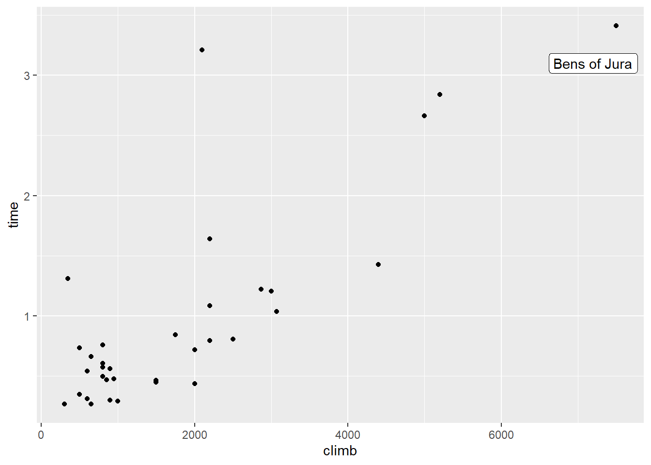
We might suspect that the elevation gain during a race could help us predict the completion time – probably courses with more of a climb take longer to finish. But before we do any sort of regression, let’s look at the data:
data(hills)
hills %>% ggplot() +
  geom_point(aes(x = climb, y = time))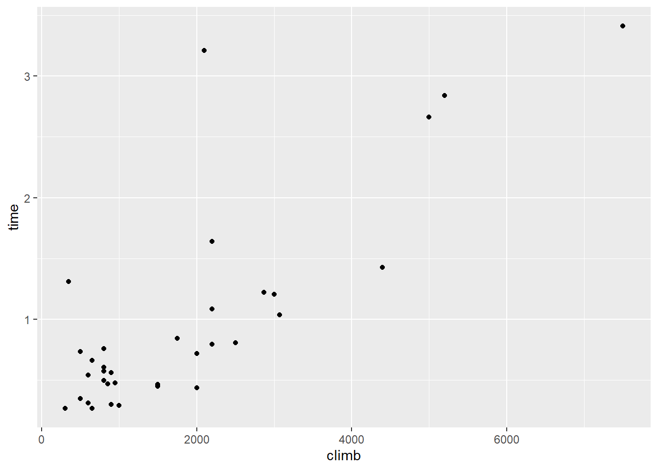
Now this is…interesting. Let’s focus first on that point with around 2000 feet of climb. You know the one I mean.
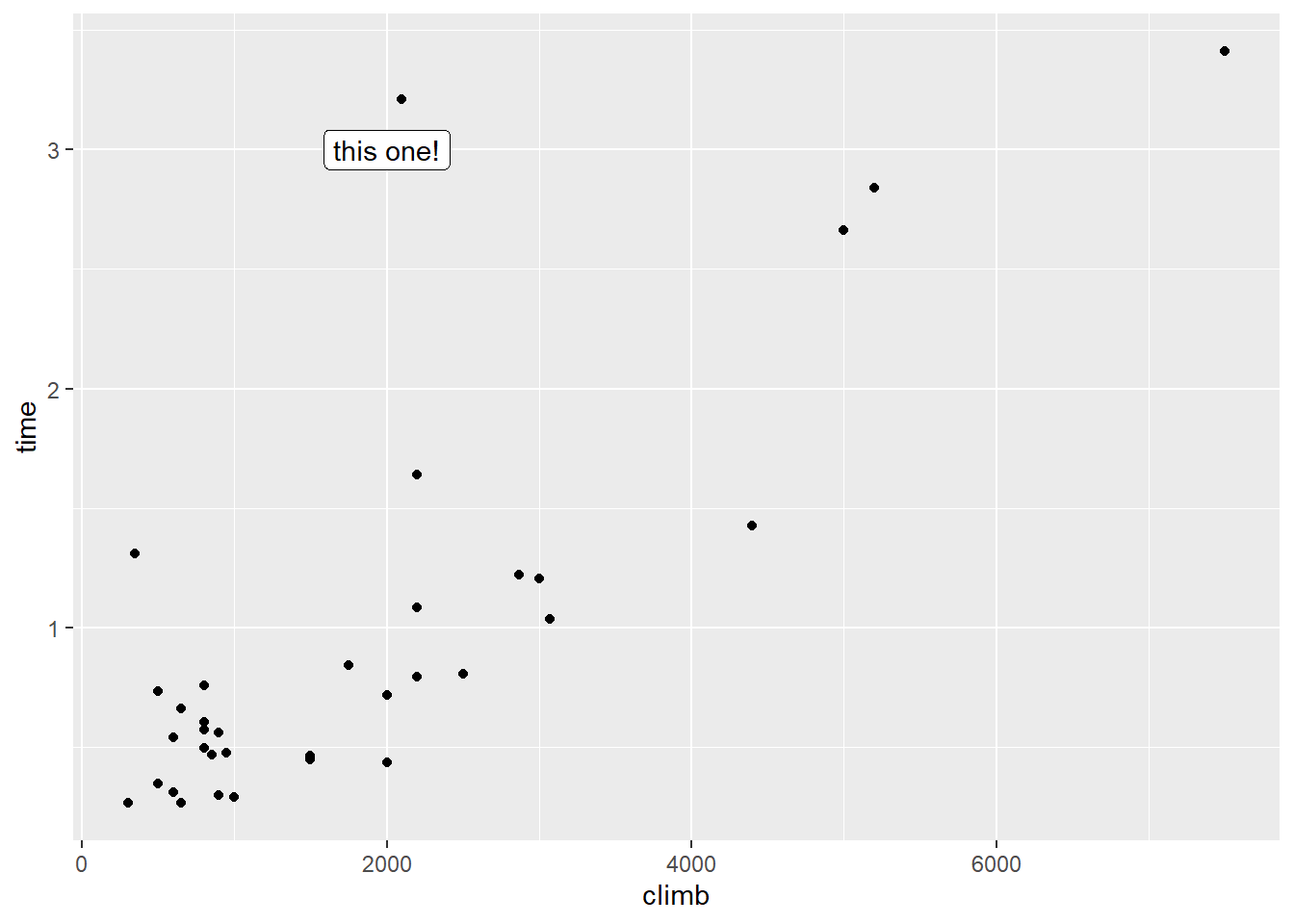
This point has a somewhat unusually high \(y\) value – that is, the record time for this course is unusually long. But that’s not what makes it an outlier. What makes it an outlier is that the record time is unusually long for a course with this amount of climb.
So this course’s time is a long way from what we’d expect given its climb. Well, we have a term for the difference between the \(\widehat{y}\) we expected and the \(y\) we observed: the residual! This point’s residual is, indeed, very large.
Let’s look at the plot of the residuals vs. the fitted values, the \(\widehat{y}\)’s.
hill_lm = lm(time ~ climb, data = hills)
hill_lm %>% plot(which = 1)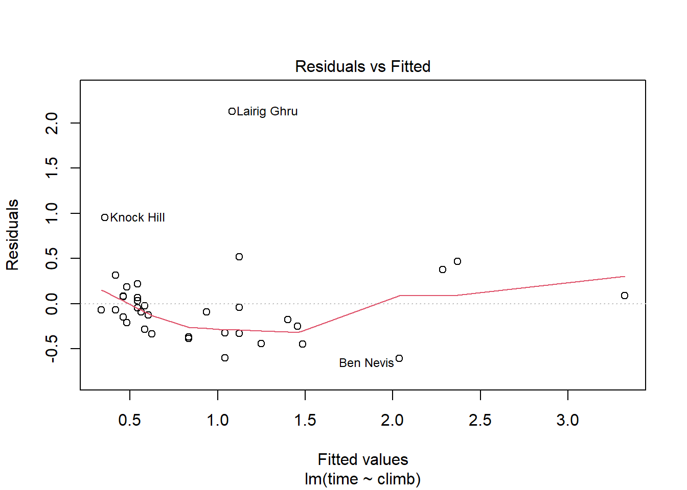
Or we can look at the Normal QQ plot of the residuals:
hill_lm %>% plot(which = 2)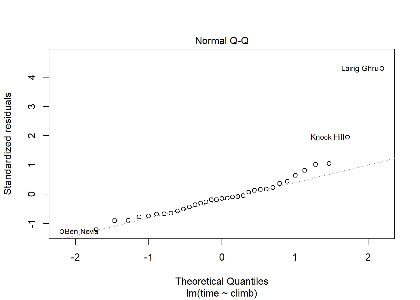
That outlier shows up with a very large residual compared to all the other points. We even get a name for it: Lairig Ghru, which is the name of the region used for the course.

Figure 1.1: Yeah, that could take a while
1.10.2 Leverage
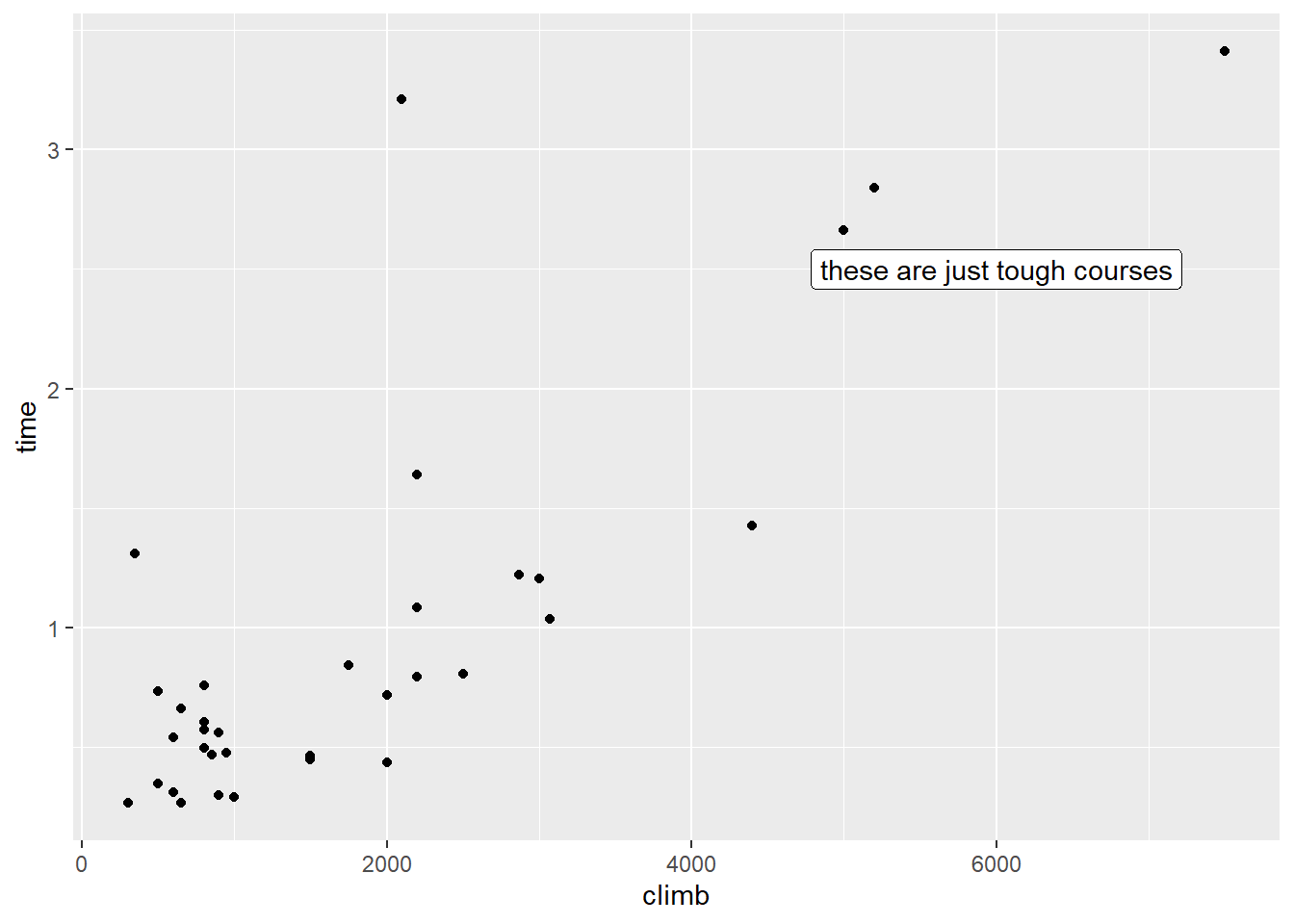
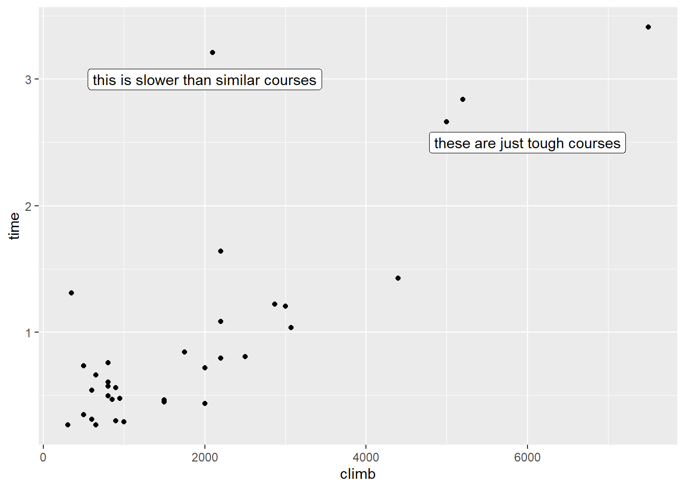
Let’s take another look at that scatterplot. This time, note the point way out in the top right corner:
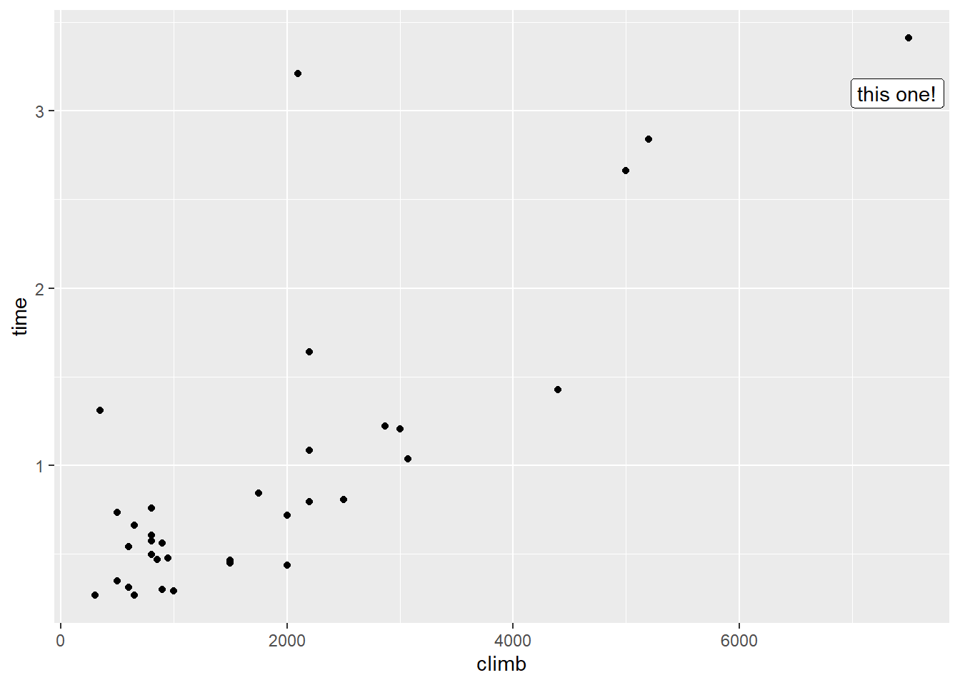
Is this point an outlier? Well, sort of. It is unusual in terms of its \(y\) value, but notice that it’s also very unusual in terms of its \(x\) value – the climb involved in this course is much higher than average.
Such a point – one with an unusual value of a predictor – is called a high-leverage point. There’s a mathematical definition for this that we won’t go into here, but you can spot high-leverage points using the scatterplot. And R actually has a function that calculates the leverage of each and every point:
hill_lm %>% hatvalues() %>% sort(decreasing = TRUE) %>% head()## Bens of Jura Two Breweries Moffat Chase Ben Nevis Kildcon Hill Knock Hill
## 0.39111445 0.15709516 0.14235506 0.10351978 0.05433180 0.05265984This super-high-climb course is the Bens of Jura.

Figure 1.2: Pretty sure you have to go over both of those
Remember, the regression line has to go through \((\overline{x}, \overline{y})\). So in a sense this is like the fulcrum of a lever. If we take a point whose \(x\) is close to \(\overline{x}\) and move it up or down, it won’t shift the slope of the line much. But if we take a point with a very far-out \(x\) value and move it up or down, it can “pull” the line with it.
Why do we call these leverage points? Well, in a sense, these points have the power – the leverage – to potentially change the slope of the line. But do they change the slope of the line? That’s a question of not just leverage, but influence.
1.10.3 Influence
An influential point is one that, well, has influence on the regression. It makes a difference if that point is in the dataset or not. Maybe having it there changes the slope of the line, or the \(R^2\) – the goodness of fit. For example, let’s take Lairig Ghru, our first outlier with an unusually long record time. First, we’ll fit a version of the model without Lairig Ghru in the dataset:
which(rownames(hills) == "Lairig Ghru")## [1] 11 # this tells me Lairig Ghru is case no. 11
hill_lm_no_LG = lm(time ~ climb, data = hills,
subset = -11)
# using "subset" fits the model using a subset of the dataWhat happens to the coefficients?
hill_lm$coefficients## (Intercept) climb
## 0.2116592755 0.0004147733hill_lm_no_LG$coefficients## (Intercept) climb
## 0.161714880 0.000407769Doesn’t seem like a super huge difference, although you have to consider that the climb coefficient is operating on a very small scale (those units are “hours per foot!”).
What about the goodness of fit?
hill_lm %>% summary() %>% .$r.squared## [1] 0.6484168hill_lm_no_LG %>% summary() %>% .$r.squared## [1] 0.8023795Ooh. The \(R^2\) is considerably higher when we take Lairig Ghru out of the dataset. And that makes sense: our model was really bad at explaining the record time for that course. With it gone, our model does better at explaining the record times overall. But Lairig Ghru didn’t have a lot of leverage, so it didn’t have that much of an effect on the slope.
Not every outlier is influential, and not every high-leverage point is influential. Generally speaking, a point has to be both an outlier and have a fair amount of leverage to be influential. But, as ever, there are no hard rules: any odd or special-looking point is worth investigating.
R has yet another handy built-in plot that can help us look at this:
hill_lm %>% plot(which = 5)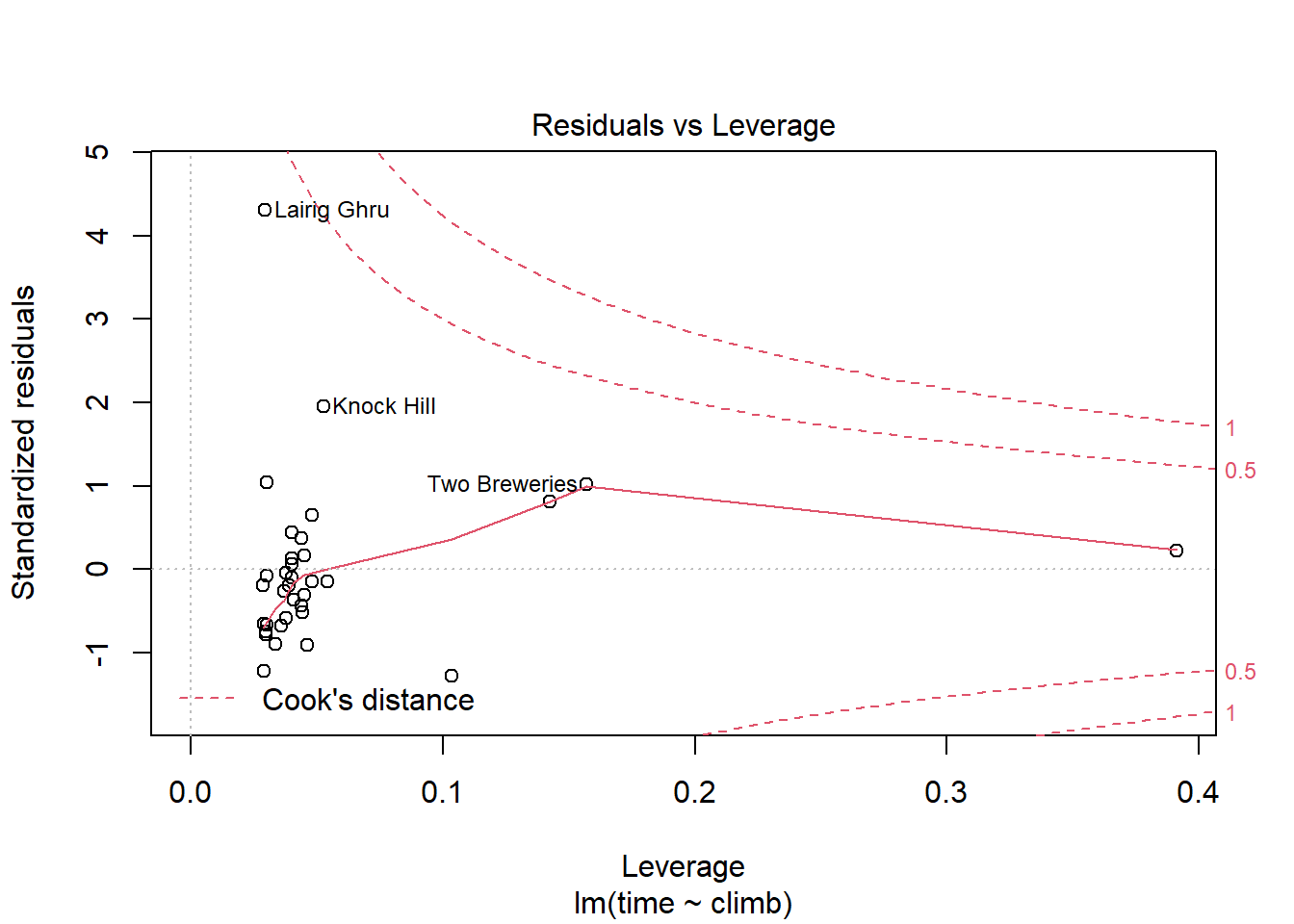
Here, the \(x\) axis shows each case’s leverage, and the \(y\) axis shows the z-score of the case’s residual. You can see that Lairig Ghru does have a really high residual – a z-score of over 4! – but not a lot of leverage.
But the Bens of Jura, way out at the right there, has a lot of leverage but a very small residual. So it may not be influential. Let’s check by fitting the model without it:
which(rownames(hills) == "Bens of Jura")## [1] 7 # this tells me Bens of Jura is case no. 7
hill_lm_no_Bens = lm(time ~ climb, data = hills,
subset = -7)
# using "subset" fits the model using a subset of the dataWhat happens to the coefficients? Not too much:
hill_lm$coefficients## (Intercept) climb
## 0.2116592755 0.0004147733hill_lm_no_Bens$coefficients## (Intercept) climb
## 0.2242361494 0.0004055751What about \(R^2\)?
hill_lm %>% summary() %>% .$r.squared## [1] 0.6484168hill_lm_no_Bens %>% summary() %>% .$r.squared## [1] 0.5253836Turns out, \(R^2\) is noticeably lower without the Bens of Jura in there. Why?
Because that course’s \(y\) value is so large, it adds a lot to the overall variation in \(y\). But meanwhile, the regression line actually does quite well at predicting the record time for that course:
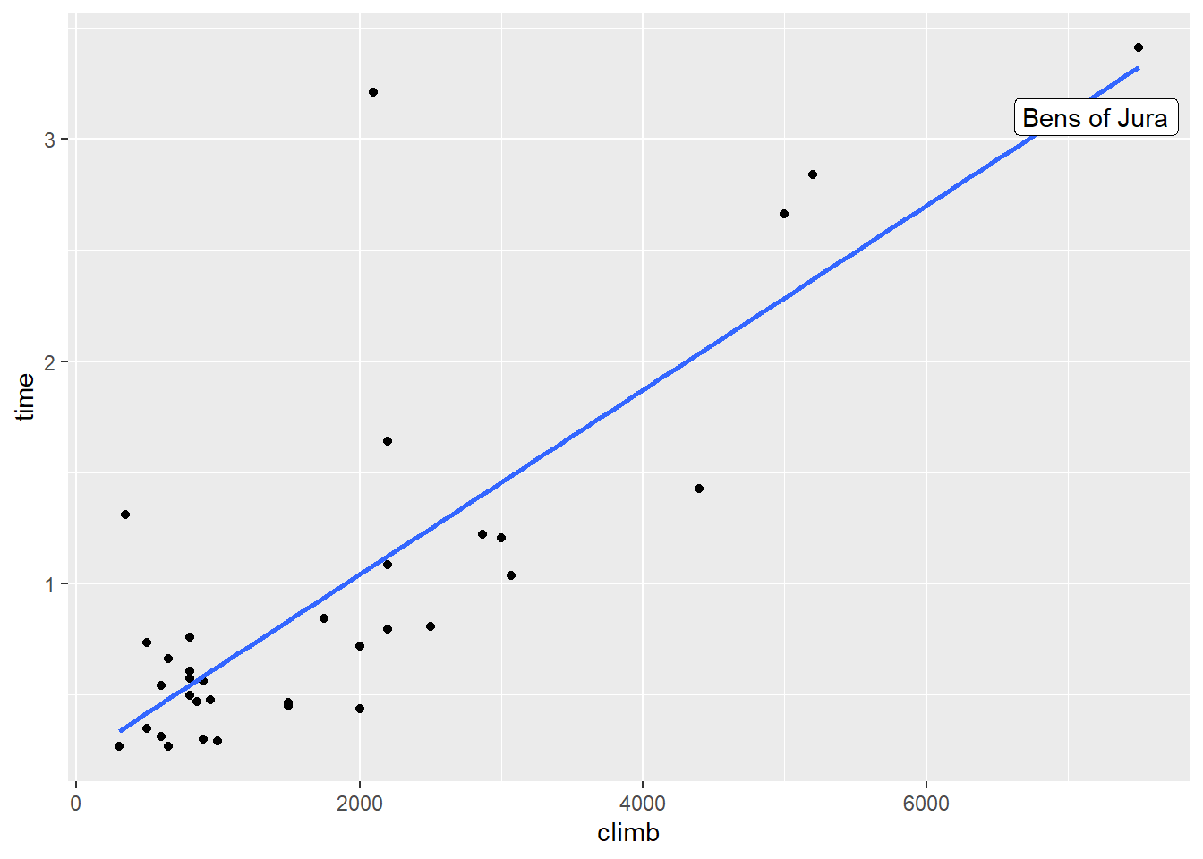
So its residual is quite small – it doesn’t increase the spread of the residuals, \(s_e\). Basically, this course adds a lot to the variation in \(y\), but the model explains almost all of it. So the proportion of the total variation in \(y\) that’s explained by the model goes up!
In general, very high-leverage points will often have this effect. So it’s something to watch for: even if your \(R^2\) looks high, you want to make sure it’s not just high because your model succeeds at predicting one really extreme case.
1.10.4 Dealing with it
So what do you do with these special points? Well, the first thing to do is to check your data. Was there a recording error somewhere? Did the lab equipment break down? Do these cases actually belong in the dataset?
For example, if I accidentally threw the Boston Marathon into the hill-racing dataset, it would be a bit of an outlying point – only about 600 feet of climb, but a record time right around 2 hours. The Boston Marathon doesn’t belong in this dataset; it’s not the same kind of race. And you might be able to catch this by looking at outliers in the dataset and seeing where they come from.
Ask me about John Snow sometime for a great story about the importance of outliers!
No, not Jon Snow. I know nothing about that guy.
If you don’t see a reason to discard the data point, try doing what we’ve already done here: try your analysis both with and without it. Does it make a difference to your conclusions? If it doesn’t, cool, fine, leave it in there. Who knows? Maybe your reader might be able to figure out why it’s anomalous. Maybe not; anomalies happen.
If the data point does make a difference to your conclusions, then you’re in a bit of a sticky spot. If at all possible, you should present both versions of the results – with and without the point. You can make a recommendation about which results you think are more appropriate, but give your reader all the information. If you have to present a single result, try your best to talk with other statisticians and subject-matter experts to decide which version to report. And mention that outliers or influential points have been removed – or left in place – when describing those results.
Response moment: Suppose that your favorite super-speed superhero decides to go race the Bens of Jura course. Afterward, the record time for the Bens of Jura is now 0.1 hours. What do you think will happen to the regression coefficients? The goodness of fit? (Who is your favorite super-speed superhero, anyway?)