4.10 Degrees of freedom
4.10.1 Introduction
So let’s talk about degrees of freedom. This is a phrase you’ve heard before – it comes up in intro stats – but my experience is that you don’t really have to think about what it means at that point. But it does show up in a lot of places, so it doesn’t hurt to get a better intuition for it.
Here’s what I assume you’ve heard about degrees of freedom: \(t\) distributions (and F distributions, if you’ve seen those) have degrees of freedom. You have to specify the degrees of freedom in order to know which \(t\) distribution you’re talking about, the way you have to specify the mean and variance for a normal distribution. Probably you learned that when you’re doing inference on a mean you use a \(t_{n-1}\) distribution, where \(n\) is the sample size. Then for inference on a simple linear regression you use \(t_{n-2}\), and for multiple linear regression you use \(t_{n-k-1}\), where \(k\) is the number of predictors in your model. Also, you may have some vague sense that more degrees of freedom is a good thing. But very possibly you never thought about why.
So what are degrees of freedom? In a general sense, they are values that exist – and can be changed – independently of one another, hence the “freedom” part. If you have a dataset with \(n\) observations with independent errors, you start with \(n\) degrees of freedom. Any model that you fit also has some number of degrees of freedom – one for each parameter that can be estimated separately from the others. The model “uses up” the df from your dataset when it finds the parameter estimates.
4.10.2 Example time!
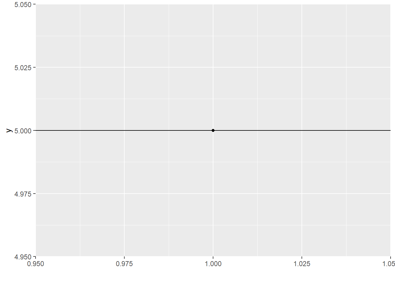
Let’s start small. Consider a very, very simple model: a horizontal line.

This horizontal-line model has one degree of freedom, because there’s exactly one thing about it I can change: the \(y\) intercept. (Secretly, of course, “fitting the best horizontal line” is just finding the mean: the best value for the \(y\) intercept is the mean of the points.)
I can fit this model to a dataset consisting of one point:
But once I do that, I have no idea how good my model is. I mean, it explains my current sample perfectly, but if I took a different sample, would I get a different horizontal line? How different? Who knows?
My model has used up the one degree of freedom provided by my dataset, and there’s nothing left over for anything else – like trying to estimate error.
Okay, let’s get a larger dataset: two points (woo!). I can fit my horizontal-line model:

Aha! Now I have the fitted \(y\)-intercept value, and I also have some information about how wrong it’s likely to be, based on how well it fits my current sample. I can do a \(t\)-test at this point if I want:
t.test(data_2pt$y)##
## One Sample t-test
##
## data: data_2pt$y
## t = 6, df = 1, p-value = 0.1051
## alternative hypothesis: true mean is not equal to 0
## 95 percent confidence interval:
## -6.706205 18.706205
## sample estimates:
## mean of x
## 6See that df=1? I had a dataset with 2 df, I used up 1 by setting the \(y\)-intercept (aka the mean) to its best possible fitted value, and then I had 1 left.
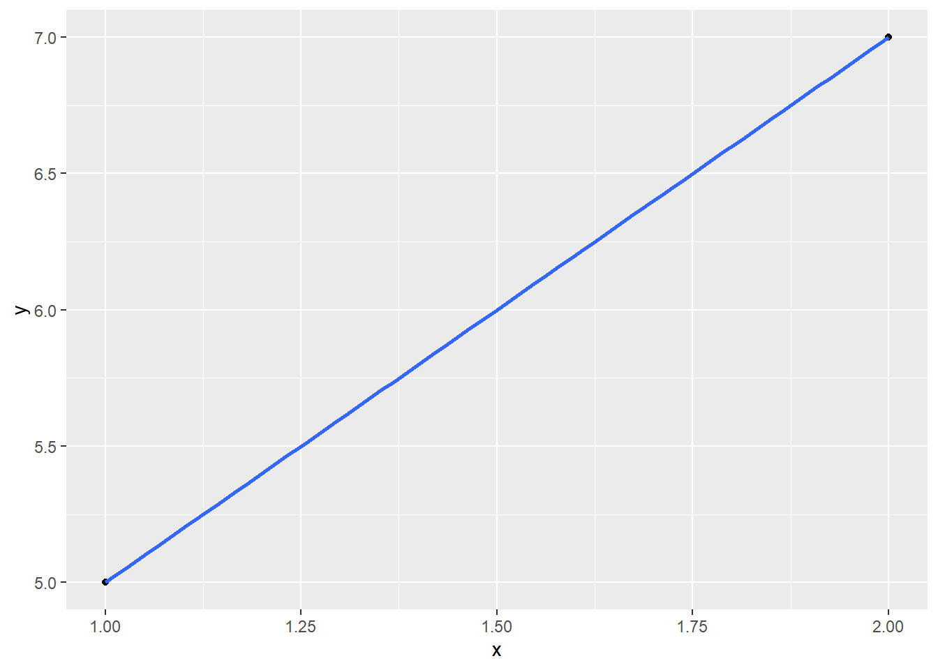
Now what if I want to get fancy and fit an actual regression line? This model has two parameters, or in other words, two things I can change in order to get the best possible fit: the intercept, and the slope. So it uses two degrees of freedom.
Response moment: What would happen if I tried to fit this model on a dataset that contains only 1 point? What if I try to fit it on a dataset with 2 points?
Let’s fit this model to my two-point dataset:
You may say: Prof T, this is ridiculous. What kind of person would try to fit two parameters using two data points?
To which I say: you. When you do experimental design.
And you may say: But…fitting two parameters with one data point?
And I say: It’s going to get weird.
As we saw before: it fits the sampled points perfectly, but I have no idea how wrong it really is – there’s no way to guess the error. That’s because, yet again, I used up all my degrees of freedom while fitting the model.
It may help to think of it this way: you can always fit a line perfectly to any two points. No matter how wildly varying the population values are, if you only sample two of them, your model fit is going to be perfect. Only by sampling a third point can you have any idea of how the population values vary – whether they are actually tightly grouped around a line, or widely scattered.
But if I have three data points, I can use two degrees of freedom to fit the model (intercept and slope) and still have one left over to give me a sense of the error:
data_3pt = data.frame(x = c(1,2,3), y = c(5,7,12))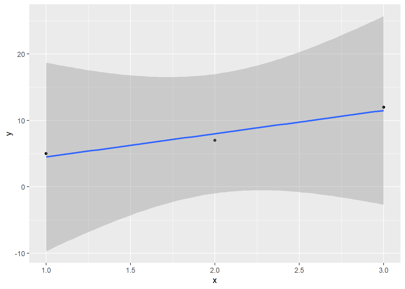
lm(y~x, data = data_3pt) %>% summary()##
## Call:
## lm(formula = y ~ x, data = data_3pt)
##
## Residuals:
## 1 2 3
## 0.5 -1.0 0.5
##
## Coefficients:
## Estimate Std. Error t value Pr(>|t|)
## (Intercept) 1.000 1.871 0.535 0.687
## x 3.500 0.866 4.041 0.154
##
## Residual standard error: 1.225 on 1 degrees of freedom
## Multiple R-squared: 0.9423, Adjusted R-squared: 0.8846
## F-statistic: 16.33 on 1 and 1 DF, p-value: 0.1544There’s the familiar old lm() summary data! And it warns us: it only had 1 degree of freedom to use to estimate the residual standard error (which underlies all the other standard errors).
4.10.3 The benefits of extra df
Take a look at that p-value for the slope: not significant. Even though the fitted slope looks quite different from 0, we have very little information about how wrong it is – just one df-worth. We’d have a better guess if we had more points:
data_4pt = data.frame(x = c(1,2,3,2.5), y = c(5,7,12,8))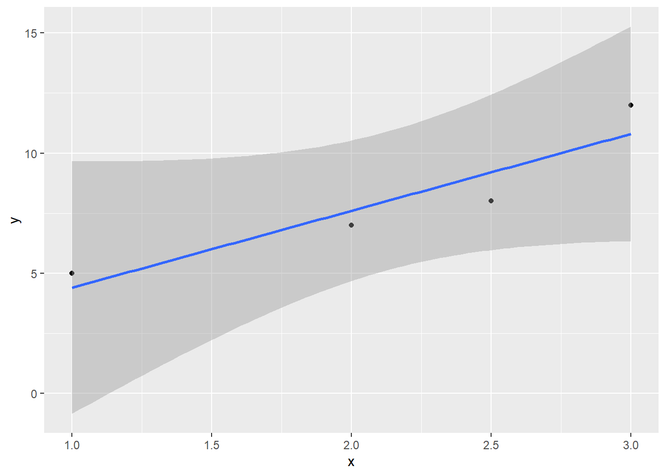
If you want to know more about why this works, check the side note!
How does this work mathematically? That’s where the df of the \(t\) distribution comes in.
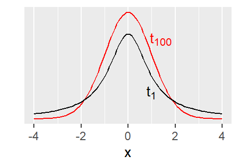
A \(t\) distribution with low df has very heavy tails and wide spread, so the critical values are waaaay out there. That makes the resulting confidence intervals very wide. And it’s hard to get a test statistic larger than the critical value.
But as the df increase, the \(t\) distribution becomes “better behaved,” with narrower tails. (You may have previously seen that a \(t_{\infty}\) is the same as a normal distribution.) The associated critical values are closer to 0, the CIs are narrower, the p-values are smaller.

…The T-800 looks a bit different.
##
## Call:
## lm(formula = y ~ x, data = data_4pt)
##
## Residuals:
##    1    2    3    4
##  0.6 -0.6  1.2 -1.2
##
## Coefficients:
##             Estimate Std. Error t value Pr(>|t|)
## (Intercept)   1.2000     2.0410   0.588   0.6161
## x             3.2000     0.9071   3.528   0.0718 .
## ---
## Signif. codes:  0 '***' 0.001 '**' 0.01 '*' 0.05 '.' 0.1 ' ' 1
##
## Residual standard error: 1.342 on 2 degrees of freedom
## Multiple R-squared:  0.8615, Adjusted R-squared:  0.7923
## F-statistic: 12.44 on 1 and 2 DF,  p-value: 0.07181
The estimate of the slope is actually closer to 0 now, and the estimated residual standard error is higher. But! We are more sure about it, because we have a better estimate of the amount of variation in the population. So we are more confident that the real slope isn’t 0.
This is the power (pun intended) of degrees of freedom. The more you have in your dataset, the more parameters you’re able to estimate – and the more certain you can be about how well those estimates match the truth.