1.6 Simple Linear Regression Fundamentals

Correlation is a nice way of talking about the direction and strength of a relationship between two quantitative variables. But it has its limits. Suppose I’m telling you about cars, and I tell you that the correlation between a car’s horsepower and its quarter-mile time is -0.70. Well, now you know that cars with higher horsepower tend to have faster quarter-mile times, and you know that the relationship is moderately strong but not that strong. But if I tell you a car has 150 horsepower, you have no idea what that means about its quarter-mile time. You know there is a relationship, but not exactly what it is.

That’s where linear regression comes in. Instead of just talking about the strength of the linear relationship between the variables, let’s actually find out what line it is.

1.6.1 Describing a relationship

Here’s the horsepower and quarter-mile time measurements for 30 different models of cars:

cars.new = my_cars %>%
  filter(hp < 300,
         qsec < 22)
cars.new %>%
  ggplot() +
  geom_point(aes(x = hp,y = qsec))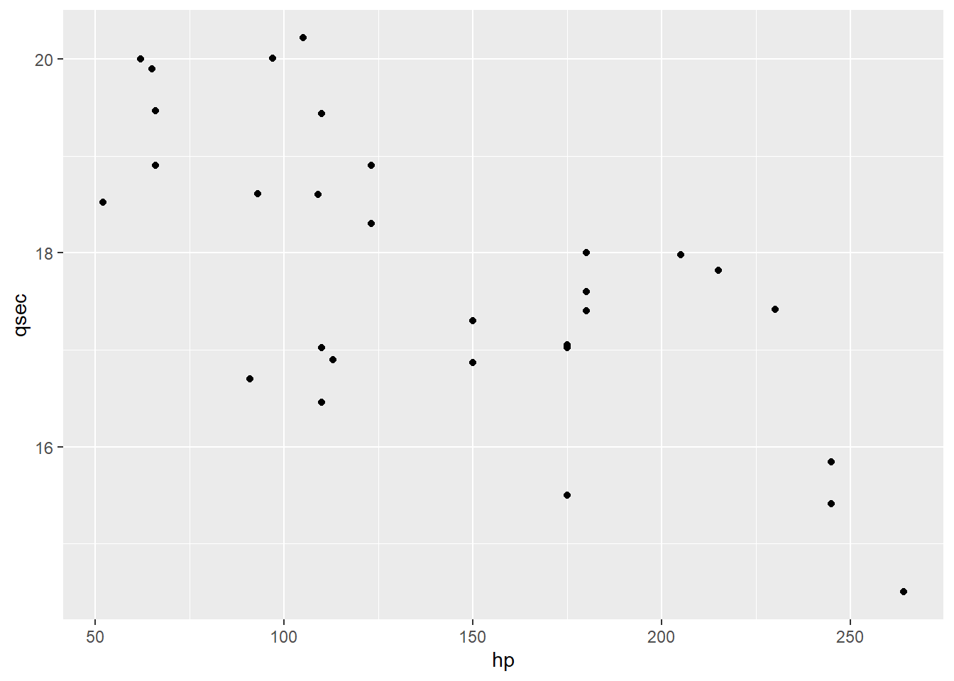

What we want to do is draw a line to describe the relationship between these variables.

Now, obviously, we can’t draw a single straight line that hits all these points. But we can draw a line that sort of…gets as close as possible. Like this one:

cars.new %>%
  ggplot(aes(x = hp,y = qsec)) +
  geom_point() +
  geom_smooth(method = 'lm', se = FALSE)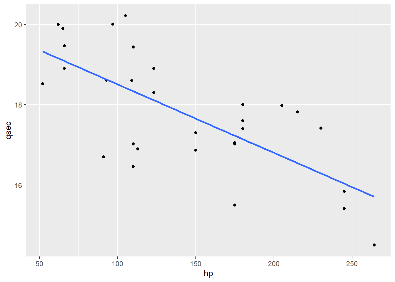

1.6.2 The linear regression equation

So how do we describe this line? You may recall from days past that in order to describe a straight line we need two pieces of information. In particular, we’ll use the line’s y-intercept and its slope.

We can use these to write the equation of a generic line:

\[\hat{y} = b_0 + b_1 x\]

Or, if we plug in the variables we’re interested in:

\[\widehat{qsec} = b_0 + b_1 hp\]

Here, \(qsec\) is the response variable and \(hp\) is the predictor variable; \(b_0\) is the intercept, and \(b_1\) is the slope (in particular, the slope associated with the predictor \(hp\)).

We can use R to find the best possible coefficients for this line – the intercept and slope that work the best. (We’ll talk about what “best” means a little later.) This uses the lm function, which stands for “linear model.”

lm(qsec ~ hp, data = cars.new)

## 
## Call:
## lm(formula = qsec ~ hp, data = cars.new)
## 
## Coefficients:
## (Intercept)           hp  
##    20.21384     -0.01706

So the fitted or estimated regression equation is:

\[\widehat{qsec} = 20.2 - 0.017 hp\]

Note the little hats on \(y\) and \(qsec\) here. That’s an indication that something is a predicted value. This equation describes the line through the points overall, but it isn’t necessarily going to pass exactly through any given point.

For example, we have a couple of cars in the dataset with 150 horsepower. If we plug in 150 for \(hp\) in the equation, we get:

20.2 - 0.017*150

## [1] 17.65

That’s what we would predict for those cars’ quarter-mile times, if they were right on the line. But it’s wrong:

cars.new %>%
  filter(hp == 150) %>%
  dplyr::select(qsec)

##    qsec
## 1 16.87
## 2 17.30

For both of these cars, \(\widehat{qsec} = 17.65\), but the actual observed value of \(qsec\) is 16.87 for one car, and 17.30 for the other. The discrepancy \(qsec - \widehat{qsec}\) is called the residual for that point.

There’s nothing inherently wrong with this. Again, our line couldn’t possibly go right through all the points. It’s just picking up the general trend.

1.6.3 Interpreting coefficients

We have a generic form of the regression equation, and we’ve found the best possible values for each coefficient.

\[\widehat{qsec} = b_0 + b_1 hp\] \[\widehat{qsec} = 20.2 - 0.017 hp\]

So how do we interpret these regression coefficients?

Let’s start with the \(y\) intercept. By definition, this is where the line crosses the \(y\) axis: it’s the predicted \(y\) value when \(x=0\). In our context, this is what we’d predict as the quarter-mile time for a car with…0 horsepower.

This is not particularly enlightening. Often, the intercept isn’t that interesting in and of itself: it’s not unusual that 0 doesn’t even make sense as a value of your predictor. It’s just important mathematically, in order to know where to put the line.

The slope is more directly interesting. We can interpret this as “change in \(\hat{y}\) per unit change in \(x\).” In context, that means that for a car with 1 additional horsepower, we predict its quarter-mile time will be 0.017 seconds faster.

Now, 0.017 seconds may not sound like a lot! But you have to consider the scale. These cars have, roughly, 50 to 250 horsepower. A one-unit change in horsepower is pretty tiny, so the change in the predicted response is also tiny. When you interpret regression coefficients, you have to think about the scale for each variable before you decide whether the slope is large.

1.6.4 Regression caution

We’ll have a lot more to say about the assumptions and conditions for regression when we start using it for inference. But even right now, when we’re just using it as a descriptive tool, it’s important to remember that it has some limitations.

For starters, just like correlation, linear regression is linear. It’s right there in the name! We are drawing a straight line through the points. If the actual relationship between the variables isn’t linear, our model can’t do a good job of describing it.

It’s also worth noting that regression (and correlation too, actually) can be affected by outliers. This is also something we’ll explore more later, but for now, bear in mind that if there are extreme or outlying points in the dataset, they may pull the line around so that it doesn’t fit the rest of the points as well.

All of which is to say: it’s really important to look at your data! Don’t just throw your variables into lm and grab the regression coefficients. Check a scatterplot for potential problems, and make sure that regression is actually the right tool for the job.

Response moment: Think about direction, form, and strength. Which of these does the regression line reflect? Which does it not reflect? What does it assume?