Chapter 13 Bayesian Analysis of Rates

Poisson distributions are often used to model the number of “relatively rare” events that occur over a certain interval of time. In a Poisson distribution situation, the length of the time interval is fixed, e.g., earthquakes in an hour, births in a day, accidents in a week, home runs in a baseball game. Given data on time intervals of this fixed length, we measure the number of events that happen in each interval

Now we will estimate the rate at which events happen by measuring the time that elapses between events. Exponential distributions are often used to model waiting times between “relatively rare” events that occur over time.

An Exponential distribution is a special case of a Gamma distribution with shape parameter $\alpha=1$. A continuous RV $Y$ has an Exponential distribution with rate parameter³⁰ $\theta>0$ if its density satisfies \[\begin{align*} f(y|\theta) & = \theta e^{-\theta y}, \qquad y>0. \end{align*}\]

In R: dexp(y, rate) for density, rexp to simulate, qexp for quantiles, etc.

Here we are using the symbol $\theta$ rather than $\lambda$ to represent the rate parameter because $\theta$ will be the parameter of interest in analysis of data on waiting times from an Exponential distribution.

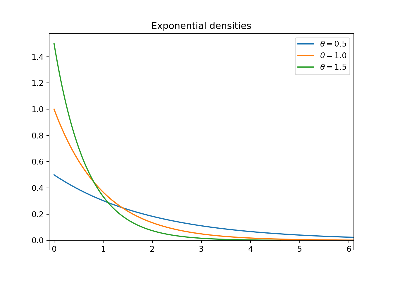
It can be shown that an Exponential($\theta$) density has \[\begin{align*} \text{Mean (EV)} & = \frac{1}{\theta}\\ \text{Variance} & = \frac{1}{\theta^2} \\ \text{Mode} & = 0,\\ \text{Median} & = \frac{\log(2)}{\theta} \approx \frac{0.693}{\theta} \end{align*}\]

Exponential distributions are often used to model waiting times between events. Data values are measured in units of time, e.g., minutes, hours, etc.

$\theta$ is the rate at which events occur over time (e.g., 2 per hour on average)
$1/\theta$ is the mean time between events (e.g., 1/2 hour on average)

Exponential distributions have many nice properties, including the following.

Cumulative waiting time follows a Gamma distribution. If $Y_1$ and $Y_2$ are independent, $Y_1$ has an Exponential($\theta$) distribution, and $Y_2$ has an Exponential($\theta$) distribution, then $Y_1+Y_2$ has a Gamma distribution³¹ with shape parameter 2 and rate parameter $\theta$. For example, if $Y_1$ represents the waiting time until the first event, and $Y_2$ represents the additional waiting time until the second event, then $Y_1+Y_2$ is the total waiting time until 2 events occurs, and $Y_1+Y_2$ follows a Gamma(2, $\theta$) distribution. This result extends naturally to more than two events. If $Y_1, Y_2, \ldots, Y_n$ are independent, each with an Exponential($\theta$) distribution, then $(Y_1+\cdots +Y_n)$ follows a Gamma($n$, $\theta$) distribution. Including the normalizing constant, the Gamma($n$, $\theta$) density is \[ f(y|\theta) = \frac{\theta^n}{(n-1)!}y^{n - 1}e^{-\theta y}, \qquad y>0 \]

Time rescaling. If $Y$ has an Exponential distribution with rate parameter $\theta$ and $c>0$ is a constant, then $cY$ has an Exponential distribution with rate parameter $\theta/c$. For example, if $Y$ is measured in hours with rate 2 per hour (and mean 1/2 hour), then $60Y$ is measured in minutes with rate 2/60 per minute (and mean 60/2 minutes).

Example 13.1 Suppose that times (measured in hours, including fractions of an hour) between earthquakes of any magnitude in Southern California follow an Exponential distribution with mean $\theta$. We wish to estimate the rate at which earthquakes occur $\theta$, that is, the average number of earthquakes per hour.

Sketch your prior distribution for $\theta$ and describe its features. What are the possible values of $\theta$? Does $\theta$ take values on a discrete or continuous scale?
As usual, we’ll start with a discrete prior for $\theta$ to illustrate ideas.

$\theta$ 0.25 0.50 0.75 1.00 1.25

Prior probability 0.04 0.16 0.25 0.29 0.26

Suppose a single earthquake with a waiting time of 3.2 hours is observed. Determine the likelihood column of the Bayes table. Find the posterior distribution of $\theta$. For what values of $\theta$ is the posterior probability greater than the prior probability? Why?
Now suppose a second wait time of 1.6 hours is observed, independently of the first. Find the posterior distribution of $\theta$ after observing these two wait times, using the posterior distribution from the previous part as the prior distribution in this part.
Now consider the original prior again. Find the posterior distribution of $\theta$ after observing a wait time of 3.2 hours for the first earthquake and 1.6 hours for the second, without the intermediate updating of the posterior after the first earthquake. How does the likelihood column relate to the likelihood columns from the previous parts? How does the posterior distribution compare with the posterior distribution from the previous part?
Now consider the original prior again. Suppose that instead of observing the two individual values, we only observe that there is a total of wait time of 4.8 hours for 2 earthquakes. Find the posterior distribution of $\theta$. In particular, how do you determine the likelihood column? How does the likelihood column compare to the one from the previous part? How does posterior compare to the previous part?
Suppose we wait for another earthquake. How could you use simulation to approximate the posterior predictive distribution of the waiting time?
Now let’s consider a continuous Gamma(4, 3) prior distribution for $\theta$. Use grid approximation to compute the posterior distribution of $\theta$ given a single wait time of 3.2 hours. Plot the prior, (scaled) likelihood, and posterior. (Note: you will need to cut the grid off at some point. While $\theta$ can take any value greater than 0, the interval [0, 5] accounts for 99.98% of the prior probability.)
Now let’s consider some real data. Assume that waiting times between earthquakes (of any magnitude) in Southern California follow an Exponential distribution with rate $\theta$. Assume a Gamma(4, 3) prior distribution for $\theta$. The following summarizes data for a sample of 100 earthquakes³². There was a total waiting time of 63.09 hours for the 100 earthquakes. Use grid approximation to compute the posterior distribution of $\theta$ given the data. Be sure to specify the likelihood. Plot the prior, (scaled) likelihood, and posterior.
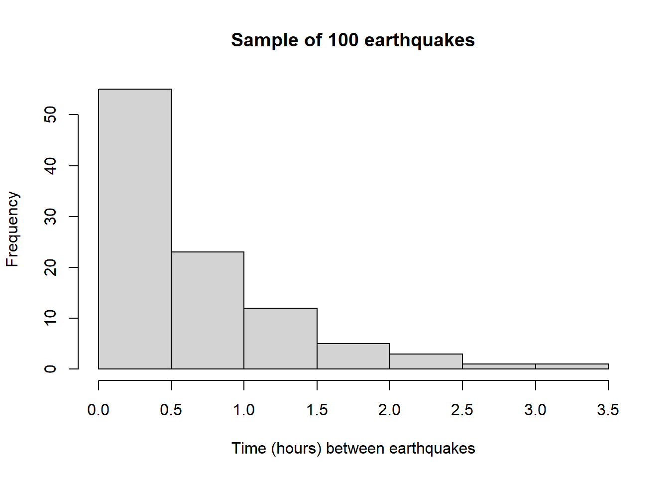
```
##      Min.   1st Qu.    Median      Mean   3rd Qu.      Max. 
## 0.0008222 0.1263917 0.4572944 0.6308882 0.9394931 3.0761806
```
```
## [1] 0.6417422
```

\(\theta\)	0.25	0.50	0.75	1.00	1.25
Prior probability	0.04	0.16	0.25	0.29	0.26

Solution. to Example 13.1

Your prior is whatever it is. We’ll discuss how we chose a prior in a later part. The parameter $\theta$ is the average rate at which earthquakes occur per hour, which takes values on a continuous scale.

The likelihood is the Exponential($\theta$) density evaluated at $y=3.2$, computed for each value of $\theta$. \[ f(y=3.2|\theta) = \theta e^{-3.2\theta} \]

For example, the likelihood of $y=3.2$ when $\theta=0.25$ is $0.25 e^{-3.2(0.25)}=0.11$. As always posterior is proportional to the product of prior and likelihood. Remember that $\theta$ represents the rate, so smaller values of $\theta$ correspond to longer average wait times. Observing a wait time of 3.2 places greater probability on $\theta = 0.25$ (mean wait of 4 hours) and $\theta=0.5$ (mean wait of 2 hours) relative to prior.

theta	prior	likelihood	product	posterior
0.25	0.04	0.1123	0.0045	0.0811
0.50	0.16	0.1009	0.0162	0.2914
0.75	0.25	0.0680	0.0170	0.3069
1.00	0.29	0.0408	0.0118	0.2133
1.25	0.26	0.0229	0.0060	0.1074

The likelihood is the Exponential($\theta$) density evaluated at $y=1.6$, computed for each value of $\theta$. \[ f(y=1.6|\theta) = \theta e^{-1.6\theta} \]

For example, the likelihood of $y=1.6$ when $\theta=0.25$ is $0.25 e^{-1.6(0.25)}=0.168$. As always posterior is proportional to the product of prior and likelihood. The posterior distribution after these two earthquakes is similar to the posterior after the first earthquake, though the SD is a little smaller.

theta	prior	likelihood	product	posterior
0.25	0.0811	0.1676	0.0136	0.0648
0.50	0.2914	0.2247	0.0655	0.3123
0.75	0.3069	0.2259	0.0693	0.3307
1.00	0.2133	0.2019	0.0431	0.2054
1.25	0.1074	0.1692	0.0182	0.0867

Since the earthquakes are independent the likelihood is the product of the likelihoods from the two previous parts \[\begin{align*} f(y=(3.2, 1.6)|\theta) & = \left(\theta e^{-3.2\theta}\right)\left(\theta e^{-1.6\theta}\right)\\ & = \theta^2 e^{-4.8\theta} \end{align*}\]

For example, the likelihood for $\theta=0.25$ is $0.25^2e ^{-4.8(0.25)} = 0.0188$. Unsurprisingly, the posterior distribution is the same as in the previous part.

theta	prior	likelihood	product	posterior
0.25	0.04	0.0188	0.0008	0.0648
0.50	0.16	0.0227	0.0036	0.3123
0.75	0.25	0.0154	0.0038	0.3307
1.00	0.29	0.0082	0.0024	0.2054
1.25	0.26	0.0039	0.0010	0.0867

By the Gamma property of cumulative times, the total time until 2 earthquakes follows a Gamma distribution with shape parameter 2 and rate parameter $\theta$. The likelihood is the Gamma density evaluated at a value of 4.8 (total wait time for 2 earthquakes) computed for each value of $\theta$. \[\begin{align*} f(\bar{y}=4.8/2|\theta) & = \frac{\theta^2}{(2-1)!}{4.8}^{2-1}e^{-4.8\theta}\\ & \propto \theta^2 e^{-4.8\theta} \end{align*}\]

For example, the likelihood for $\theta=0.25$ is $\frac{0.25^2}{(2-1)!}{4.8}^{2-1}e^{-4.8(0.25)} = 0.09$. The likelihood is not the same as in the previous part because there are more samples of size two that yield a total wait time of 4.8 hours than those that yield a pair of wait times of 3.2 and 1.6. However, the likelihoods are proportionally the same. For example, the likelihood for $\theta=1.00$ is about 2.12 times greater than the likelihood for $\theta = 1.25$ in both this part and the previous part. Therefore, the posterior distribution is the same as in the previous part.

theta	prior	likelihood	product	posterior
0.25	0.04	0.0904	0.0036	0.0648
0.50	0.16	0.1089	0.0174	0.3123
0.75	0.25	0.0738	0.0184	0.3307
1.00	0.29	0.0395	0.0115	0.2054
1.25	0.26	0.0186	0.0048	0.0867

Simulate a value of $\theta$ from its posterior distribution and then given $\theta$ simulate a value of $Y$ from an Exponential($\theta$) distribution, and repeat many times. Summarize the simulated $Y$ values to approximate the posterior predictive distribution. (We’ll see some code a little later.)

For each value of $\theta$ in the grid compute the prior probability \[ \pi(\theta) \propto \theta^{4 -1}e^{-3\theta}, \qquad \theta > 0 \] The prior mean of the rate parameter $\theta$ is 4/3 = 1.333 earthquakes per hour.

The likelihood is the Exponential($\theta$) density evaluated at $y=3.2$, computed for each value of $\theta$ in the grid. \[ f(y=3.2|\theta) = \theta e^{-3.2\theta} \] The likelihood is maximized at the observed sample rate of 1/3.2 = 0.3125 earthquakes per hour.

# prior
theta = seq(0, 5, 0.001)

prior = dgamma(theta, shape = 4, rate = 3)
prior = prior / sum(prior)

# data
n = 1 # sample size
y = 3.2 # sample mean

# likelihood
likelihood = dexp(y, theta)

# posterior
product = likelihood * prior
posterior = product / sum(product)

ylim = c(0, max(c(prior, posterior, likelihood / sum(likelihood))))
xlim = range(theta)
plot(theta, prior, type='l', xlim=xlim, ylim=ylim, col="orange", xlab='theta', ylab='', yaxt='n')
par(new=T) 
plot(theta, likelihood/sum(likelihood), type='l', xlim=xlim, ylim=ylim, col="skyblue", xlab='', ylab='', yaxt='n')
par(new=T)
plot(theta, posterior, type='l', xlim=xlim, ylim=ylim, col="seagreen", xlab='', ylab='', yaxt='n')
legend("topright", c("prior", "scaled likelihood", "posterior"), lty=1, col=c("orange", "skyblue", "seagreen"))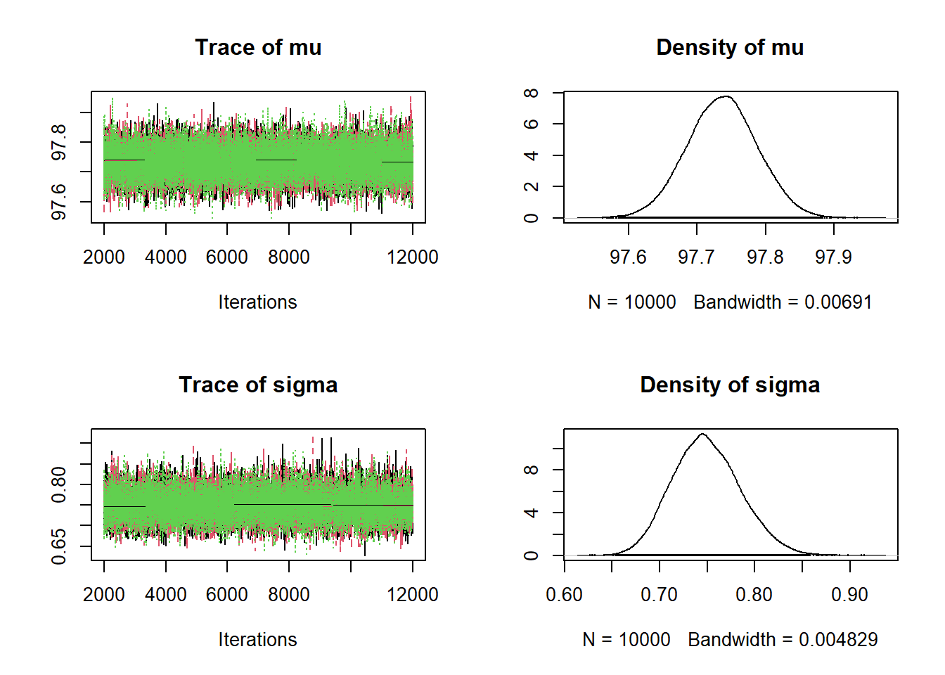

The total wait time for 100 earthquakes follows a Gamma distribution with shape parameter 100 and rate parameter $\theta$. The likelihood is the Gamma(100, $\theta$) density evaluated at a value of 63.09 (for the wait time for the 100 earthquakes) computed for each $\theta$. \[\begin{align*} f(\bar{y}=63.09 / 100|\theta) & = \frac{\theta^{100}}{(100-1)!}{63.09}^{100-1}e^{-63.09\theta}\\ & \propto \theta^{100} e^{-63.09\theta} \end{align*}\]

The sample mean time between earthquakes is 63.09/100 = 0.63 hours (about 38 minutes). The likelihood is centered at the sample rate of 100/63.09 = 1.59 earthquakes per hour. The posterior distribution follows the likelihood fairly closely.

# prior
theta = seq(0, 5, 0.001)

prior = dgamma(theta, shape = 4, rate = 3)
prior = prior / sum(prior)

# data
n = 100 # sample size
y = 63.09 / 100 # sample mean

# likelihood - for total time
likelihood = dgamma(n * y, shape = n, rate = theta)

# posterior
product = likelihood * prior
posterior = product / sum(product)

ylim = c(0, max(c(prior, posterior, likelihood / sum(likelihood))))
xlim = range(theta)
plot(theta, prior, type='l', xlim=xlim, ylim=ylim, col="orange", xlab='theta', ylab='', yaxt='n')
par(new=T) 
plot(theta, likelihood/sum(likelihood), type='l', xlim=xlim, ylim=ylim, col="skyblue", xlab='', ylab='', yaxt='n')
par(new=T)
plot(theta, posterior, type='l', xlim=xlim, ylim=ylim, col="seagreen", xlab='', ylab='', yaxt='n')
legend("topright", c("prior", "scaled likelihood", "posterior"), lty=1, col=c("orange", "skyblue", "seagreen"))

In Bayesian analysis of the rare parameter $\theta$ of an Exponential distribution, Gamma distributions are commonly used as prior distributions.

Example 13.2 Suppose that times (measured in hours, including fractions of an hour) between earthquakes of any magnitude in Southern California follow an Exponential distribution with mean $\theta$. We wish to estimate the rate at which earthquakes occur $\theta$, that is, the average number of earthquakes per hour. Assume a Gamma prior distribution for $\theta$ with prior mean 4/3 and prior SD 2/3.

Identify prior density $\pi(\theta)$. Plot the prior distribution. Find a prior 95% credible interval for $\theta$.
Suppose a single wait time of 3.2 hours is observed. Write the likelihood function.
Write an expression for the posterior distribution of $\theta$ given a single wait time of 3.2 hours. Identify by the name the posterior distribution and the values of relevant parameters. Plot the prior distribution, (scaled) likelihood, and posterior distribution. Find the posterior mean, posterior SD, and a posterior 95% credible interval for $\theta$.
Now consider the original prior again. Determine the likelihood of observing a wait time of 3.2 hours for the first earthquake and a wait time of 1.6 hours for the second. Find the posterior distribution of $\theta$ given this sample. Identify by the name the posterior distribution and the values of relevant parameters. Plot the prior distribution, (scaled) likelihood, and posterior distribution. Find the posterior mean, posterior SD, and a posterior 95% credible interval for $\theta$.
Consider the original prior again. Determine the likelihood of observing a total wait time until two earthquakes of 4.8 hours. Find the posterior distribution of $\theta$ given this sample. Identify by the name the posterior distribution and the values of relevant parameters. How does this compare to the previous part?
Consider the data on a sample of 100 earthquakes in the total wait time ws 63.09 hours. Determine the likelihood function. Find the posterior distribution of $\theta$ given this sample. Identify by the name the posterior distribution and the values of relevant parameters. Plot the prior distribution, (scaled) likelihood, and posterior distribution. Find the posterior mean, posterior SD, and a posterior 95% credible interval for $\theta$.
Interpret the credible interval from the previous part in context.
Express the posterior mean of $\theta$ based on the data as a weighted average of the prior mean and the sample mean.

Solution. to Example 13.2

If the prior mean is $\mu = 4/3$ and the prior SD is $\sigma = 2/3$, then \[\begin{align*} \lambda & = \frac{\mu}{\sigma^2} & & = \frac{4/3}{(2/3)^2} = 3\\ \alpha & = \mu\lambda & & (4/3)(3) = 4 \end{align*}\] Remember that in the Gamma(4,3) prior distribution $\theta$ is treated as the variable. \[ \pi(\theta) \propto \theta^{4-1}e^{-3\theta}, \qquad \theta > 0. \]

This is the same prior we used in the grid approximation in Example 13.1. See below for a plot. Use qgamma for find the endpoints of a 95% prior credible interval.
```
qgamma(c(0.025, 0.975), shape = 4, rate = 3)
```
```
## [1] 0.3632885 2.9224244
```
The likelihood is the Exponential($\theta$) density evaluated at $y=3.2$, computed for each value of $\theta$. \[ f(y=3.2|\theta) = \theta e^{-3.2\theta}, \qquad \theta > 0 \]

Posterior is proportional to likelihood times prior \[\begin{align*} \pi(\theta|y = 3.2) & \propto \left(\theta e^{-3.2\theta}\right)\left(\theta^{4-1}e^{-3\theta}\right), \qquad \theta > 0,\\ & \propto \theta^{(4 + 1) - 1}e^{-(3+3.2)\theta}, \qquad \theta > 0. \end{align*}\]

We recognize the above as the Gamma density with shape parameter $\alpha=4+1$ and rate parameter $\lambda = 3 + 3.2$.

\[\begin{align*} \text{Posterior mean } & = \frac{\alpha}{\lambda} & & \frac{5}{6.2} = 0.806\\ \text{Posterior SD} & = \sqrt{\frac{\alpha}{\lambda^2}} & & \sqrt{\frac{5}{6.2^2}} = 0.361 \end{align*}\]

qgamma(c(0.025, 0.975), shape = 4 + 1, rate = 3 + 3.2)

## [1] 0.2618526 1.6518691

theta = seq(0, 5, 0.001) # the grid is just for plotting

# prior
alpha = 4
lambda = 3
prior = dgamma(theta, shape = alpha, rate = lambda)

# likelihood
n = 1 # sample size
y = 3.2 # sample mean
likelihood = dexp(y, theta)

# posterior
posterior = dgamma(theta, alpha + n, lambda + n * y)

# plot
plot_continuous_posterior <- function(theta, prior, likelihood, posterior) {

  ymax = max(c(prior, posterior))

  scaled_likelihood = likelihood * ymax / max(likelihood)

  plot(theta, prior, type='l', col='orange', xlim= range(theta), ylim=c(0, ymax), ylab='', yaxt='n')
  par(new=T)
  plot(theta, scaled_likelihood, type='l', col='skyblue', xlim=range(theta), ylim=c(0, ymax), ylab='',  yaxt='n')
  par(new=T)
  plot(theta, posterior, type='l', col='seagreen', xlim=range(theta), ylim=c(0, ymax), ylab='', yaxt='n')
  legend("topright", c("prior", "scaled likelihood", "posterior"), lty=1, col=c("orange", "skyblue", "seagreen"))
}

plot_continuous_posterior(theta, prior, likelihood, posterior)

abline(v = qgamma(c(0.025, 0.975), alpha + n, lambda + n * y),
   col = "seagreen", lty = 2)

The likelihood is the product of the likelihoods of $y=3.2$ and $y=1.6$. \[ f(y=(3.2, 1.6)|\theta) = \left(\theta e^{-3.2\theta}\right)\left(\theta e^{-1.6\theta}\right) = \theta^2 e^{-4.8\theta}, \qquad \theta>0. \]

The posterior satisfies \[\begin{align*} \pi(\theta|y = (3.2, 1.6)) & \propto \left(\theta^2 e^{-4.8\theta}\right)\left(\theta^{4-1}e^{-3\theta}\right), \qquad \theta > 0,\\ & \propto \theta^{(4 + 2) - 1}e^{-(3+4.8)\theta}, \qquad \theta > 0. \end{align*}\]

We recognize the above as the Gamma density with shape parameter $\alpha=4+2$ and rate parameter $\lambda = 3 + 4.8$.

\[\begin{align*} \text{Posterior mean } & = \frac{\alpha}{\lambda} & & \frac{6}{7.8} = 0.769\\ \text{Posterior SD} & = \sqrt{\frac{\alpha}{\lambda^2}} & & \sqrt{\frac{6}{7.8^2}} = 0.314 \end{align*}\]
```
n  = 2 # sample size
y = (3.2 + 1.6) / 2 # sample mean

# likelihood
likelihood = dexp(3.2, theta) * dexp(1.6, theta)

# posterior
posterior = dgamma(theta, alpha + n, lambda + n * y)

# plot
plot_continuous_posterior(theta, prior, likelihood, posterior)

abline(v = qgamma(c(0.025, 0.975), alpha + y, lambda + n * y),
   col = "seagreen", lty = 2)
```
By the Gamma property of cumulative times, the total time until 2 earthquakes follows a Gamma distribution with shape parameter 2 and rate parameter $\theta$. The likelihood is the Gamma density evaluated at a value of 4.8 (total wait time for 2 earthquakes) computed for each value of $\theta$. \[\begin{align*} f(\bar{y}=4.8/2|\theta) & = \frac{\theta^2}{(2-1)!}{4.8}^{2-1}e^{-4.8\theta}\\ & \propto \theta^2 e^{-4.8\theta} \end{align*}\]

The shape of the likelihood as a function of $\theta$ is the same as in the previous part; the likelihood functions are proportionally the same. Therefore, the posterior distribution is the same as in the previous part.
```
# likelihood
n = 2 # sample size
y = (3.2 + 1.6) / 2 # sample mean
likelihood = dgamma(n * y, shape = n, rate = theta)

# posterior
posterior = dgamma(theta, alpha + n, lambda + n * y)

# plot
plot_continuous_posterior(theta, prior, likelihood, posterior)

abline(v = qgamma(c(0.025, 0.975), alpha + n, lambda + n * y),
   col = "seagreen", lty = 2)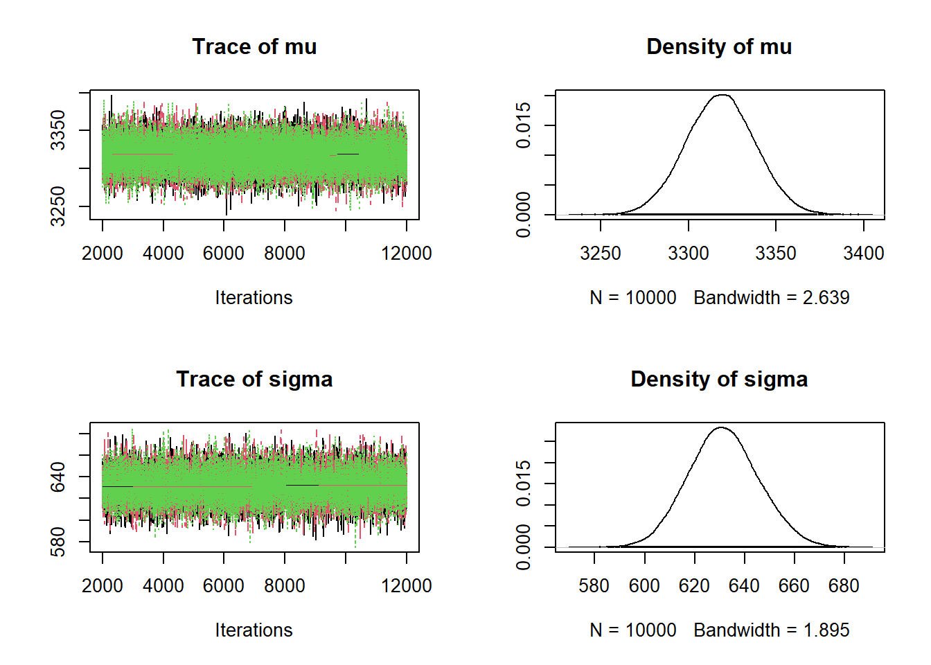
```
The total wait time for 100 earthquakes follows a Gamma distribution with shape parameter 100 and rate parameter $\theta$. The likelihood is the Gamma(100, $\theta$) density evaluated at a value of 63.09 (for the wait time for the 100 earthquakes) computed for each $\theta$. \[\begin{align*} f(\bar{y}=63.09 / 100|\theta) & = \frac{\theta^{100}}{(100-1)!}{63.09}^{100-1}e^{-63.09\theta}\\ & \propto \theta^{100} e^{-63.09\theta} \end{align*}\]

The sample mean time between earthquakes is 63.09/100 = 0.63 hours (about 38 minutes). The likelihood is centered at the sample rate of 100/63.09 = 1.59 earthquakes per hour.

The posterior satisfies \[\begin{align*} \pi(\theta|\bar{y} = 63.09/100) & \propto \left(\theta^{100} e^{-63.09\theta}\right)\left(\theta^{4-1}e^{-3\theta}\right), \qquad \theta > 0,\\ & \propto \theta^{(100 + 4) - 1}e^{-(3+63.09)\theta}, \qquad \theta > 0. \end{align*}\]

We recognize the above as the Gamma density with shape parameter $\alpha=4+100$ and rate parameter $\lambda = 3 + 63.09$. The posterior distribution follows the likelihood fairly closely.

\[\begin{align*} \text{Posterior mean } & = \frac{\alpha}{\lambda} & & \frac{104}{66.09} = 1.57\\ \text{Posterior SD} & = \sqrt{\frac{\alpha}{\lambda^2}} & & \sqrt{\frac{104}{66.09^2}} = 0.154 \end{align*}\]

The posterior distribution follows the likelihood fairly closely, but the prior still has a little influence.
```
# likelihood
n = 100 # sample size
y = 63.09 / 100 # sample mean
likelihood = dgamma(n * y, n, theta)

# posterior
posterior = dgamma(theta, alpha + n, lambda + n * y)

# plot
plot_continuous_posterior(theta, prior, likelihood, posterior)

abline(v = qgamma(c(0.025, 0.975), alpha + n, lambda + n * y),
   col = "seagreen", lty = 2)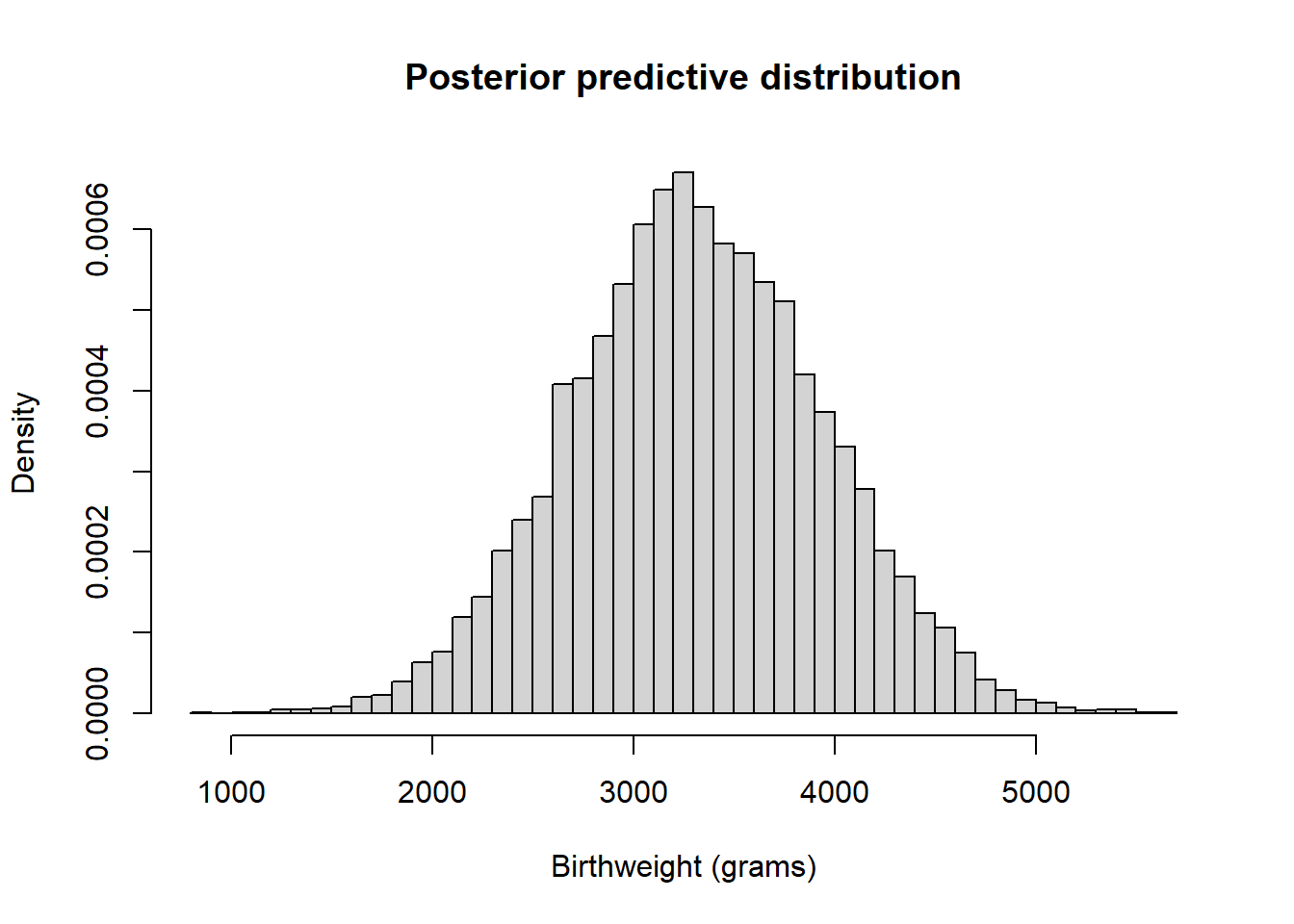
```
```
qgamma(c(0.025, 0.975), alpha + n, lambda + n * y)
```
```
## [1] 1.285755 1.890111
```
There is a posterior probability of 95% that the rate at which earthquakes occur in Southern California is between 1.28 and 1.89 earthquakes per hour.
The prior mean of the rate parameter is 4/3=1.333, based on a “prior observation time” of 3 “hours.” The sample rate is 100/63.09 = 1.59, based on a sample size of 100. The posterior mean of the rate parameter is (4 + 100)/(3 + 63.09) = 1.57. The posterior mean is a weighted average of the prior mean and the sample mean with the weights based on the “sample sizes” \[ 1.57 = \frac{4+100}{3 + 63.09} = \left(\frac{3}{3 + 63.09}\right)\left(\frac{4}{3}\right) + \left(\frac{63.09}{3 + 63.09}\right)\left(\frac{100}{63.09}\right) = (0.045)(1.333)+ (0.955)(1.585) \]

In the previous example we saw that if the values of the measured variable follow an Exponential distribution with rate parameter $\theta$ and the prior for $\theta$ follows a Gamma distribution, then the posterior distribution for $\theta$ given the data also follows a Gamma distribution.

Gamma-Exponential model.³³ Consider a measured variable $Y$ which, given $\theta$, follows an Exponential distribution with rate parameter $\theta$. Let $\bar{y}$ be the sample mean for a random sample of size $n$. Suppose $\theta$ has a Gamma$(\alpha, \lambda)$ prior distribution. Then the posterior distribution of $\theta$ given $\bar{y}$ is the Gamma$(\alpha+n, \lambda+n\bar{y})$ distribution.

That is, Gamma distributions form a conjugate prior family for an Exponential likelihood.

The posterior distribution is a compromise between prior and likelihood. For the Gamma-Exponential model, there is an intuitive interpretation of this compromise. In a sense, you can interpret $\alpha$ as “prior number of events” and $\lambda$ as “prior total observation time,” but these are only “pseudo-observations.” Also, $\alpha$ and $\lambda$ are not necessarily integers. (Be careful not confuse this interpretation with the one for Poisson distributions.)

Note that if $\bar{y}$ is the sample mean time between events is then $n\bar{y} = \sum_{i=1}^n y_i$ is the total time of observation.

	Prior	Data	Posterior
Total count	$\alpha$	$n$	$\alpha+n$
Total time	$\lambda$	$n\bar{y}$	$\lambda + n\bar{y}$
Average rate	$\frac{\alpha}{\lambda}$	$\frac{1}{\bar{y}}$	$\frac{\alpha+n}{\lambda+n\bar{y}}$

The posterior “sample size” is the sum of the “prior sample size” $\alpha$ and the observed sample size of $n$.
The posterior “total time” is the sum of the “prior total observation time” $\lambda$ and the total observation time of $n\bar{y}$.
The posterior mean is a weighted average of the prior mean of the rate parameter $\theta$ and the sample rate ($1/\bar{y}$), with weights proportional to the “total times.”

\[ \frac{\alpha+n}{\lambda+n\bar{y}}= \frac{\lambda}{\lambda+n\bar{y}}\left(\frac{\alpha}{\lambda}\right) + \frac{n\bar{y}}{\lambda+n\bar{y}}\left(\frac{1}{\bar{y}}\right) \]

Larger values of $\lambda$ indicate stronger prior beliefs, due to smaller prior variance, and give more weight to the prior. Roughly, larger $\lambda$ means a “longer prior total observation time.”
The posterior SD generally gets smaller as more data are collected — via a longer total time of observation $n\bar{y}$. (Since the denominator below is squared, it will be large relative to the numerator). \[ \text{Posterior SD of $\theta$:} \qquad \sqrt{\frac{\alpha+n}{(\lambda+n\bar{y})^2}} \]

Rather than specifying $\alpha$ and $\beta$, a Gamma distribution prior can be specified by its prior mean and SD directly. If the prior mean is $\mu$ and the prior SD is $\sigma$, then \[\begin{align*} \lambda & = \frac{\mu}{\sigma^2}\\ \alpha & = \mu\lambda \end{align*}\]

Example 13.3 Continuing the previous example, assume that times (measured in hours, including fractions of an hour) between earthquakes of any magnitude in Southern California follow an Exponential distribution with mean $\theta$. Assume a Gamma(4, 3) prior distribution for $\theta$. Consider the sample data in which there were 100 earthquakes in 63.09 hours.

How could you use simulation to find the posterior distribution of the mean time between earthquakes. Conduct the simulation and find a central 95% posterior credible interval for the mean time between earthquakes.
Because the waiting times are skewed to the right, we might be more interested in the median time between earthquakes. How could you use simulation to find the posterior distribution of the median time between earthquakes. Conduct the simulation and find a central 95% posterior credible interval for the median time between earthquakes.
How could you use simulation (not JAGS) to approximate the posterior predictive distribution of the waiting time until the next earthquake.
Use the simulation from the previous part to find and interpret a 95% posterior prediction interval with a lower bound of 0.
Use JAGS to approximate the posterior distribution of $\theta$ given this sample. Compare with the results from the previous example.

Solution. to Example 13.3

Since $\theta$ is the rate, the mean waiting time is $1/\theta$. Therefore, we can just simulate a value of $\theta$ from its posterior distribution, find $1/\theta$ and repeat many times. There is a 95% posterior probability that the mean time between earthquakes is between 0.53 and 0.77 hours (about 32 to 46 minutes.)
```
Nrep = 10000
theta_sim = rgamma(Nrep, 104, 66.09)
hist(1 / theta_sim, freq = FALSE,
 main = "Posterior distribution of mean",
 xlab = "Mean waiting time (hours)",
 ylab = "Density")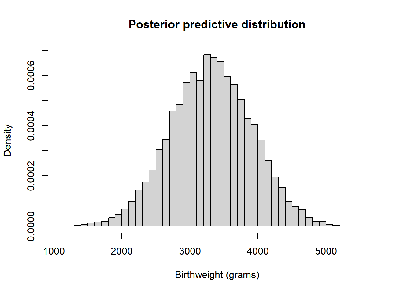
```
```
quantile(1 / theta_sim, c(0.025, 0.975))
```
```
##      2.5%     97.5% 
## 0.5293036 0.7772620
```
In general, finding the posterior distribution of the median could be tricky. But for Exponential, we have that the median is $\log(2)/\theta$. Therefore, we can just simulate a value of $\theta$ from its posterior distribution, find $\log(2)/\theta$ and repeat many times. There is a 95% posterior probability that the median time between earthquakes is between 0.37 and 0.54 hours (about 22 to 32 minutes.)
```
Nrep = 10000
theta_sim = rgamma(Nrep, 104, 66.09)
hist(log(2) / theta_sim, freq = FALSE,
 main = "Posterior distribution of median",
 xlab = "Median waiting time (hours)",
 ylab = "Density")
```
```
quantile(log(2) / theta_sim, c(0.025, 0.975))
```
```
##      2.5%     97.5% 
## 0.3675249 0.5393983
```

Simulate a value from its posterior distribution, then given $\theta$ simulate a value of $Y$ from an Exponential distribution with rate $\theta$, and repeat many times and summarizes the $Y$’s.

Nrep = 10000
theta_sim = rgamma(Nrep, 104, 66.09)
y_sim = rexp(Nrep, rate = theta_sim)
hist(y_sim, breaks = 100, freq = FALSE,
 main = "Posterior predictive distribution",
 xlab = "Waiting time (hours)",
 ylab = "Density")

quantile(y_sim, 0.95)

##      95% 
## 1.886496

There is a posterior predictive probability of 95% that the next earthquake will occur within 1.98 hours.
Roughly, for 95% of earthquakes the waiting time for the next earthquake is less than 1.98 hours.
See JAGS code below. The results are very similar to the theoretical results from the previous example.

The data has been loaded as individual values, the waiting time for each of the 100 earthquakes.
Likelihood is defined as a loop. For each y[i] value, the likelihood is computing according to a Exponential($\theta$) distribution. (If only the total time had been loaded, then this would be a Gamma likelihood.)
Prior distribution is a Gamma distribution. (Remember, JAGS syntax for dgamma, dpois, etc, is not the same as in R.)

# data
data = read.csv("_data/quakes100.csv")
y = (1 / 60) * data$Waiting.time..minutes.
n = length(y)

# model
model_string <- "model{

  # Likelihood
  for (i in 1:n){
    y[i] ~ dexp(theta)
  }

  # Prior
  theta ~ dgamma(alpha, lambda)
  alpha <- 4  
  lambda <- 3

}"

# Compile the model
dataList = list(y=y, n=n)

Nrep = 10000
Nchains = 3

model <- jags.model(textConnection(model_string), 
                    data=dataList,
                    n.chains=Nchains)

## Compiling model graph
##    Resolving undeclared variables
##    Allocating nodes
## Graph information:
##    Observed stochastic nodes: 100
##    Unobserved stochastic nodes: 1
##    Total graph size: 104
## 
## Initializing model

update(model, 1000, progress.bar="none")

posterior_sample <- coda.samples(model, 
                                 variable.names=c("theta"),
                                 n.iter=Nrep,
                                 progress.bar="none")

# Summarize and check diagnostics
summary(posterior_sample)

## 
## Iterations = 1001:11000
## Thinning interval = 1 
## Number of chains = 3 
## Sample size per chain = 10000 
## 
## 1. Empirical mean and standard deviation for each variable,
##    plus standard error of the mean:
## 
##           Mean             SD       Naive SE Time-series SE 
##      1.5736983      0.1535573      0.0008866      0.0008986 
## 
## 2. Quantiles for each variable:
## 
##  2.5%   25%   50%   75% 97.5% 
## 1.288 1.468 1.569 1.674 1.888

plot(posterior_sample)

Sometimes Exponential densities are parametrized in terms of the scale parameter $1/\theta$, so that the mean is $\theta$.↩︎
This result is a special case of the following. If $Y_1$ and $Y_2$ are independent, $Y_1$ has a Gamma($\alpha_1$, $\theta$) distribution, and $Y_2$ has a Gamma($\alpha_2$, $\theta$) distribution, then $Y_1+Y_2$ has a Gamma distribution with shape parameter $\alpha_1+\alpha_2$ and rate parameter $\theta$. The rate parameters must be the same, for otherwise the variables would be on different scales (e.g., minutes versus hours) and it wouldn’t make sense to add them.↩︎
Source: Lots of data on earthquakes can be found at https://scedc.caltech.edu/.↩︎
I’ve been naming these models in the form “Prior-Likelihood,” e.g. Gamma prior and Exponential likelihood. I would rather do it as “Likelihood-Prior.” In modeling, the likelihood comes first; what is an appropriate distributional model for the observed data? This likelihood depends on some parameters, and then a prior distribution is placed on these parameters. So in modeling the order is likelihood then prior, and it would be nice if the names followed that pattern. But “Beta-Binomial” is the canonical example, and no one calls that “Binomial-Beta.” To be consistent, we’ll stick with the “Prior-Likelihood” naming convention.↩︎

	Prior	Data	Posterior
Total count	\(\alpha\)	\(n\)	\(\alpha+n\)
Total time	\(\lambda\)	\(n\bar{y}\)	\(\lambda + n\bar{y}\)
Average rate	\(\frac{\alpha}{\lambda}\)	\(\frac{1}{\bar{y}}\)	\(\frac{\alpha+n}{\lambda+n\bar{y}}\)