19.2 Adding Levels to the Hierarchy

A hierarchical model can have several layers. In the free throw example in 18, we considered free throw percentages of individual players relative to the league-wide average free throw percentage. But suppose we want to compare the free throw percentage of individual players relative to the average free throw percentage of players of the same position (guard, forward, center), and also compare the position-by-position average free throw percentage to the overall league-wide average. For example, do guards have higher free throw percentages on average than centers?

Recall that \(\theta\) represents the free throw percentage of an individual player, while \(\mu\) represents the league-wide average. Before we assumed that for each player, \(\theta\) was drawn from a Beta distribution with mean \(\mu\). Now we will introduce an intermediate level: for a player of position \(k\), \(\theta\) will be drawn from a Beta distribution with mean \(\mu_k\), the league-wide mean for that position (\(k\)). For each position, \(\mu_k\) will be drawn from a Beta distribution with mean \(\mu_0\), the overall average. (We could let the \(\kappa\) parameter of the Beta distribution on \(\theta\) vary by position too.)

With the additional position level in the hierarchy, the model from 18 becomes the following (with somewhat sketchy notation; we have not explicitly specified all the conditional independencies). The data consist of number of free throws attempted (\(n_j\)), number of free throws made (\(y_{j|x}\)), and position (\(x\)) for each player (\(j\)).

Likelihood. For player \(j\) in position \(x\), \(y_{j|x} \sim\) Binomial\(\left(n_j, \theta_{j|x}\right)\)
Prior.
1. For player \(j\) in position \(x\), \(\theta_{j|x}\sim\) Beta\((\mu_x\kappa_x, (1-\mu_x)\kappa_x)\).
  - The prior distribution on \(\theta_{j|x}\) encapsulates our uncertainty about the free throw percentage of an individual player of position \(x\).
  - \(\mu_x\) represents the league-wide mean for position \(x\), and is our expected value for \(\theta_{j|x}\)
  - \(\kappa_x\) is the “equivalent prior sample size” relating to the strength of our beliefs about \(\theta_{j|x}\), the free throw percentage of an individual player of position \(x\).
  - Another way to think about it: \(\kappa_x\) is inversely related to the player-by-player variability for players of position \(x\).
2. For category \(x\), \(\mu_x\sim\) Beta\((\mu_0\kappa_0, (1-\mu_0)\kappa_0)\), and \(\kappa_x\sim\) Gamma\((0.1, 0.1)\)
  - The prior distribution on \(\mu_x\) encapsulates our uncertainty about the league-wide average for players of position \(x\).
  - \(\mu_0\) represents the overall league-wide average, and is our expected value for \(\mu_x\)
  - \(\kappa_0\) is the “equivalent prior sample size” relating to the strength of our beliefs about \(\mu_{x}\), the league-wide average for player of position \(x\).
  - Another way to think about it, \(\kappa_0\) is inversely related to the position-by-position variability of the position means \(\mu_x\) relative to the overall mean \(\mu_0\).
  - The prior distribution on \(\kappa_x\) encapsulates our uncertainty in the strength of our prior beliefs about \(\mu_x\). Drawing each \(\mu_x\) from the same prior distribution is like saying the degree of uncertainty in the strength of our prior beliefs for the position-by-position averages is the same for each position. (We could include hyperparameters in the distribution for \(\kappa_x\), but it seems unnecessary.)
Hyperprior. \(\mu_0, \kappa_0\) independent with \(\mu_0\sim\) Beta(15, 5) and \(\kappa_0\sim\) Gamma\((1, 0.1)\).
- Just as in 18, the prior distribution on \(\mu_0\) encapsulates our uncertainty about the overall league-wide average.

We’ll use data from the 2018-2019 NBA season available at basketball-reference. Note that some position designations have been recoded, and that the position variable needs to be coded as numbers by JAGS.

# load the data
myData = read.csv('_data/freethrows.csv', stringsAsFactors = FALSE)
myData = myData[order(myData$FTA),] # sort by number of attempts

#myData2 = myData[sample(1:nrow(myData), 50, replace=FALSE),]

# recode positions
myData[,"Pos2"] = myData$Pos
myData[myData$Pos %in% c("C", "C-PF"), "Pos2"] = "C"
myData[myData$Pos %in% c("PF", "PF-SF", "SF", "SF-PF", "SF-SG"), "Pos2"] = "F"
myData[myData$Pos %in% c("PG", "PG-SG", "SG", "SG-PF", "SG-PG", "SG-SF"), "Pos2"] = "G"
table(myData$Pos2)

## 
##   C   F   G 
##  92 180 229

aggregate(myData$FTA ~ Pos2, myData, sum, na.rm = TRUE)

##   Pos2 myData$FTA
## 1    C       9573
## 2    F      12787
## 3    G      17071

aggregate(myData$FT ~ Pos2, myData, sum, na.rm = TRUE)

##   Pos2 myData$FT
## 1    C      6823
## 2    F      9811
## 3    G     13554

aggregate(myData$FT. ~ Pos2, myData, mean, na.rm = TRUE)

##   Pos2 myData$FT.
## 1    C  0.6916023
## 2    F  0.7338343
## 3    G  0.7585885

y = myData$FT
n = myData$FTA
J = length(y) # number of players
x = as.numeric(factor(myData$Pos2)) # convert to numbers
K = length(unique(x)) # number of categories

The table displays average free throw percentage by position. The overall average free throw percentage for the 501 players is 0.737.

We now specify the hierarchical model. Below

j indexes player
k indexes position
x[j] is the position for player j
mu[x[j]] is the league-wide mean for player j’s position
the for k loop is where the prior distribution for mu[k] is specified
kappa is treated similarly to mu

# specify the model: likelihood, prior, hyperprior

model_string <- "model{

  # Likelihood
  for (j in 1:J){
    y[j] ~ dbinom(theta[j], n[j])
  }

  # Prior - now the mean for theta depends on position
  for (j in 1:J){
    theta[j] ~ dbeta(mu[x[j]] * kappa[x[j]], (1 - mu[x[j]]) * kappa[x[j]])
  }

  # For each position, draw its mean from prior distribution
  for (k in 1:K){
    mu[k] ~ dbeta(mu0 * kappa0, (1-mu0) * kappa0)
    kappa[k] ~ dgamma(0.1, 0.1)
  }

  # Hyperprior, phi=(mu, kappa)
  mu0 ~ dbeta(3, 1)
  kappa0 ~ dgamma(0.1, 0.1)
}"

dataList = list(y = y, n = n, J = J,
                x = x, K = K) # adding position info

model <- jags.model(file = textConnection(model_string), 
                    data = dataList)

## Compiling model graph
##    Resolving undeclared variables
##    Allocating nodes
## Graph information:
##    Observed stochastic nodes: 501
##    Unobserved stochastic nodes: 509
##    Total graph size: 2029
## 
## Initializing model

update(model, n.iter = 1000)

posterior_sample <- coda.samples(model,
                       variable.names = c("theta", "mu", "mu0"),
                       n.iter = 10000,
                       n.chains = 5)

Let’s first look at the posterior means and SDs for the \(\mu\) parameters.

# first four parameters are mu's
# first two statistics in summary are mean, SD
summary(posterior_sample)$statistics[1:4, 1:2]

##            Mean          SD
## mu[1] 0.7004083 0.011883603
## mu[2] 0.7486040 0.008241897
## mu[3] 0.7763920 0.007369546
## mu0   0.7204088 0.082693220

Notice that the posterior SDs of the position means are less than the SDs of the overall mean. The certainty of an estimate at a level in the hierarchy depends on how many parameter values are contributing to that level. Each of the position means has hundreds of players contributing to it directly. But the overall mean only has the three positions means contributing directly to it. In some sense, the model with position in the hierarchy utilizes the data to estimate the position means as precisely as possible, somewhat at the expense of estimating the overall mean.

posterior_sample_values = as.matrix(posterior_sample)
mu0 = posterior_sample_values[, "mu0"]
mu1 = posterior_sample_values[, "mu[1]"]
mu2 = posterior_sample_values[, "mu[2]"]
mu3 = posterior_sample_values[, "mu[3]"]

plotPost(mu0, main = "mu0")

##                  ESS      mean    median      mode hdiMass    hdiLow   hdiHigh
## Param. Val. 4186.095 0.7204088 0.7279184 0.7365543    0.95 0.5418361 0.8713205
##             compVal pGtCompVal ROPElow ROPEhigh pLtROPE pInROPE pGtROPE
## Param. Val.      NA         NA      NA       NA      NA      NA      NA

plotPost(mu1, main = "mu1")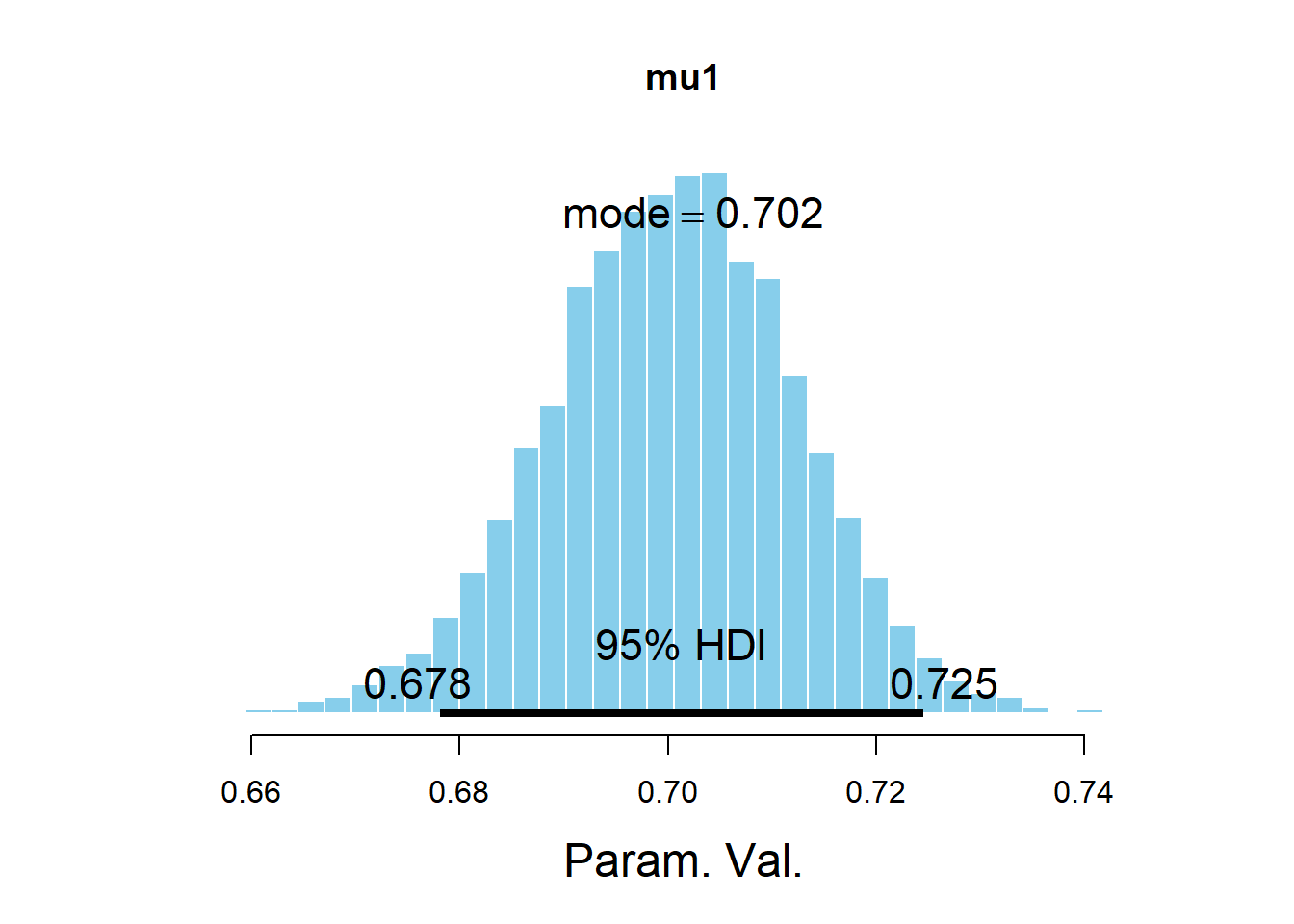

##                  ESS      mean    median      mode hdiMass    hdiLow   hdiHigh
## Param. Val. 2622.554 0.7004083 0.7006277 0.7024198    0.95 0.6780932 0.7245106
##             compVal pGtCompVal ROPElow ROPEhigh pLtROPE pInROPE pGtROPE
## Param. Val.      NA         NA      NA       NA      NA      NA      NA

plotPost(mu2, main = "mu2")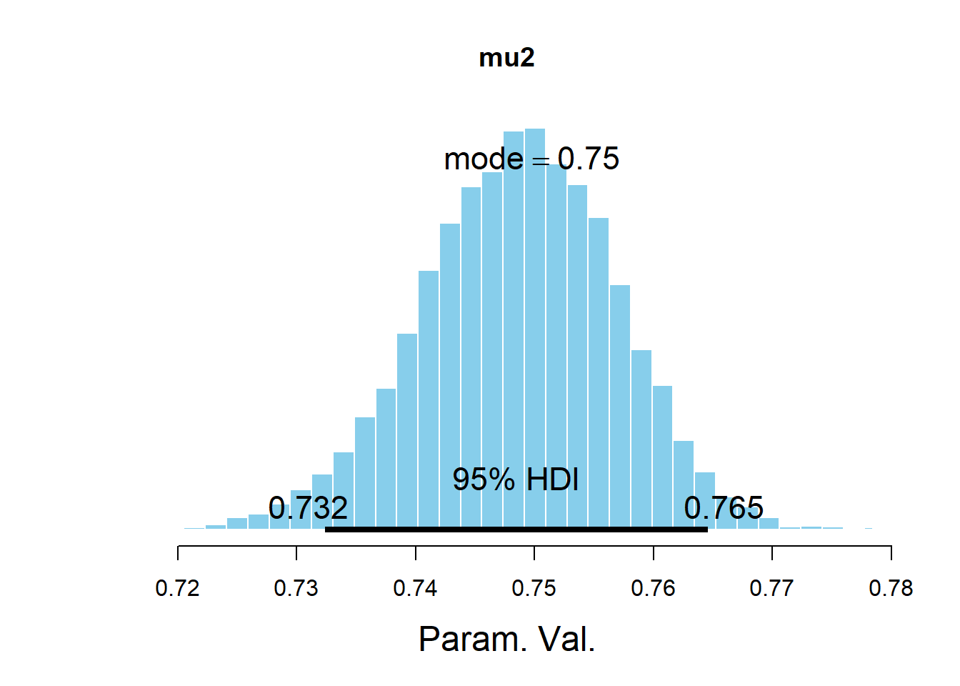

##                  ESS     mean    median      mode hdiMass    hdiLow   hdiHigh
## Param. Val. 2080.294 0.748604 0.7488376 0.7497781    0.95 0.7323842 0.7645845
##             compVal pGtCompVal ROPElow ROPEhigh pLtROPE pInROPE pGtROPE
## Param. Val.      NA         NA      NA       NA      NA      NA      NA

plotPost(mu3, main = "mu3")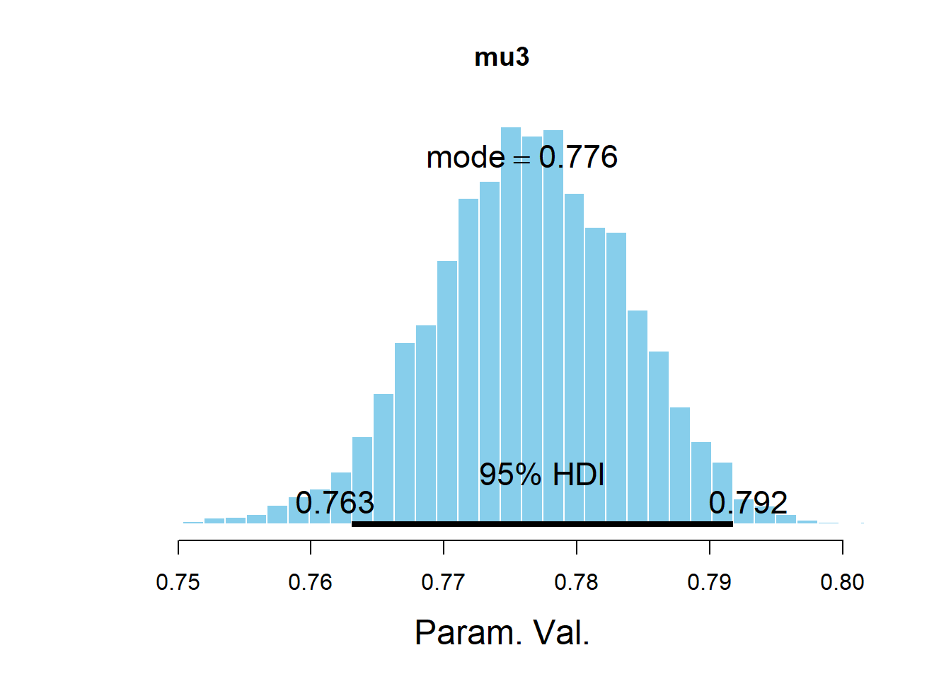

##                  ESS     mean    median      mode hdiMass    hdiLow   hdiHigh
## Param. Val. 1870.369 0.776392 0.7764682 0.7758813    0.95 0.7630633 0.7917335
##             compVal pGtCompVal ROPElow ROPEhigh pLtROPE pInROPE pGtROPE
## Param. Val.      NA         NA      NA       NA      NA      NA      NA

The code below will launch in a browser the ShinyStan GUI for exploring the results of the NBA simulation. (You’ll need to change eval to TRUE to run this code chunk.)

nba_sso <- as.shinystan(posterior_sample, model_name = "NBA Free Throws")
# nba_sso <- drop_parameters(nba_sso, pars = c("kappa", "kappa0"))
launch_shinystan(nba_sso)