19.1 Comparing Groups with a Hierarchical Model

Example 19.1 Example 17.1 which concerned whether newborns born to mothers who smoke tend to weigh less at birth than newborns from mothers who don’t smoke.

Assume birthweights follow a Normal distribution with mean $\mu_1$ for nonsmokers and mean $\mu_2$ for smokers, and standard deviation $\sigma$ . (We’re assuming a common standard deviation to simplify a little, but we could also let standard deviation vary by smoking status.)

Explain how you could model this scenario with a hierarchical model. Specify all levels in the hierarchy and the relevant parameters and distributions at each level.
Use simulation to approximate the joint and marginal prior distributions of $\mu_1$ and $\mu_2$ , and the marginal prior distribution of $\mu_1-\mu_2$ . How does the prior compare to one in Example 19.1?
Use JAGS to fit the model to the data. Summarize the joint and marginal posterior distributions of $\mu_1$ and $\mu_2$ , and the marginal posterior distribution of $\mu_1-\mu_2$ , and of the effect size. How does the posterior compare the one in Example19.1?
Do the conclusions change substantially compared to those in 19.1?

Solution. to Example 19.1

As in Example 19.1 we assume that given $\mu_1, \mu_2, \sigma$ , individual birthweights are Normally distributed with a mean that depends on smoking status: $Y_{i, x}\sim N(\mu_x, \sigma)$ . $\sigma$ represents the baby-to-baby variability in birthweights. We could have separate $\sigma$ ’s for each smoking status. Our main reason for not doing so is simplicity, and to be consistent with Example 19.1. Also to be consistent with Example 19.1 we’ll assume $(1/\sigma^2)$ has a Gamma(1, 1) prior distribution (though this isn’t the greatest choice.) Now we assume that given $\mu_0, \sigma_\mu$ , the group means $\mu_1$ and $\mu_2$ are i.i.d. $N(\mu_0, \sigma_\mu)$ . $\mu_0$ represents the overall average birthweight, and $\sigma_\mu$ represents how much the mean birthweights would vary from group to group. The hyperparameters are $\mu_0$ and $\sigma_\mu$ . The prior on $\mu_0$ represents prior uncertainty about the overall average birthweight. We’ll assume a Normal distribution prior for $\mu_0$ with prior mean 7.5 and prior SD 0.5, consistent with to be consistent with Example 19.1. $\sigma_mu$ represents how much means vary from group to group. Recall that in Example we used a prior that gave rather large credibility to no difference in means. To be somewhat consistent we’ll use an informative prior⁴⁶ which places large credibility on $\sigma_\mu$ being small, Gamma(1, 3).

While the prior distribution isn’t the same as in Example 19.1, there is still a strong prior credibility of no difference. However, we see that the prior distribution of $\mu_1-\mu_2$ has heavier tails here than it did in Example 19.1.

N = 10000

# hyperprior
mu0 = rnorm(N, 7.5, 0.5)
sigma_mu = rgamma(N, 1, 3)

# prior
mu1 = rnorm(N, mu0, sigma_mu)
mu2 = rnorm(N, mu0, sigma_mu)

theta_sim_prior = data.frame(mu0, mu1, mu2)

hist(theta_sim_prior$mu1 - theta_sim_prior$mu2, xlab = "mu1 - mu2")

ggplot(theta_sim_prior, aes(mu1, mu2)) +
  geom_point(color = "skyblue", alpha = 0.4) +
  geom_density_2d(color = "orange", size = 1) +
  geom_abline(intercept = 0, slope = 1, color="black", 
             linetype="dashed")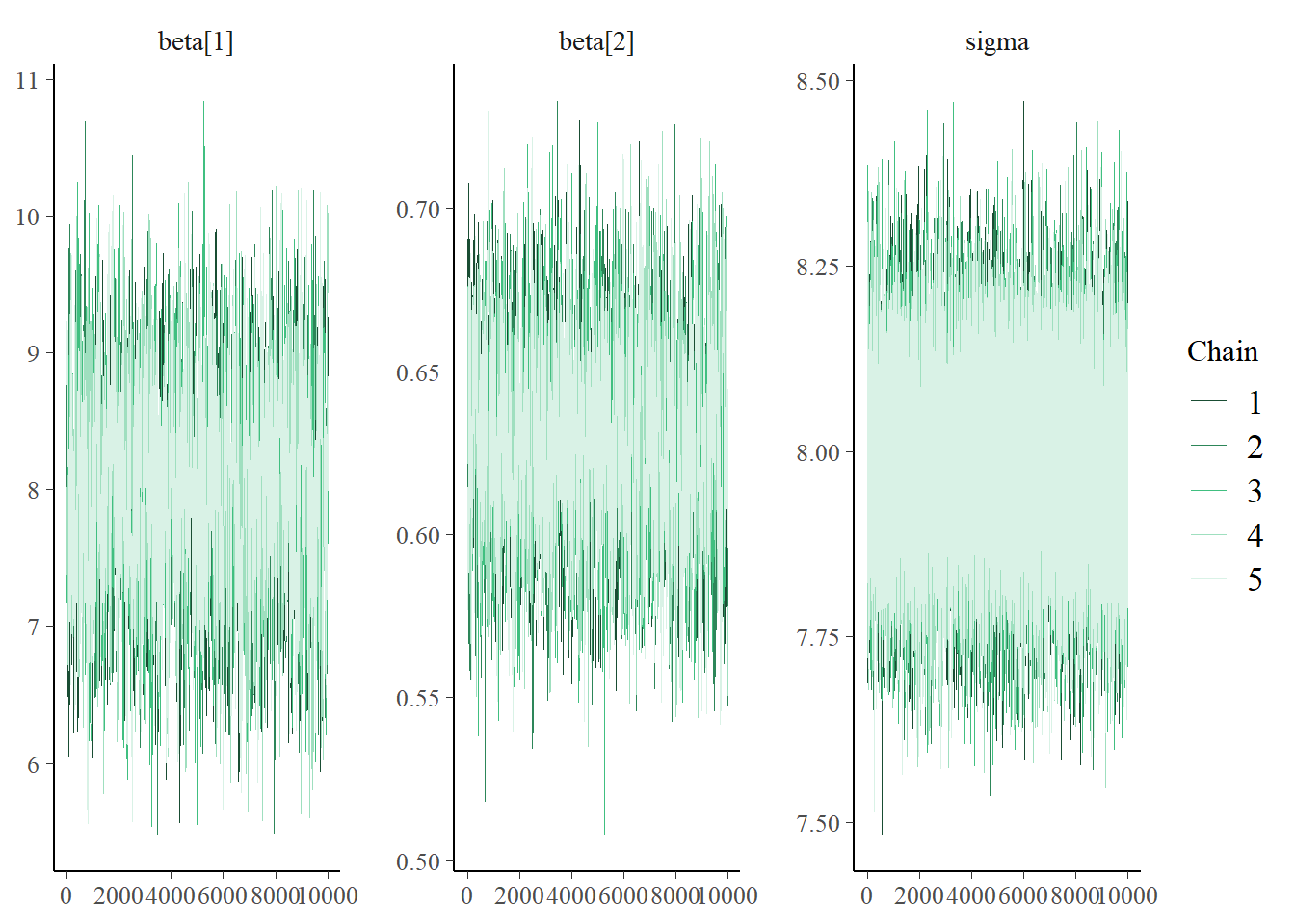

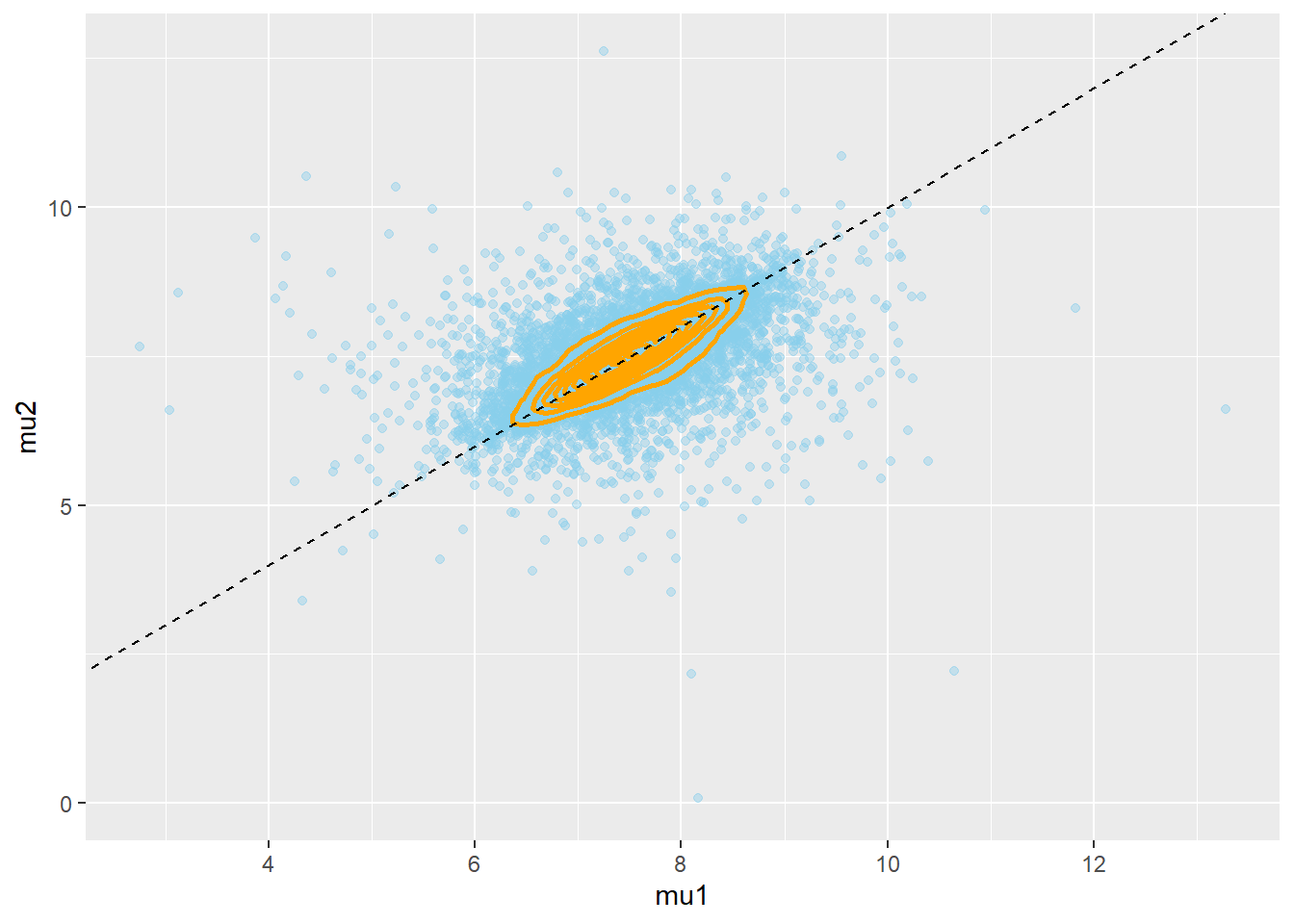
The posterior is pretty similar to the one in Example19.1. The min difference is that the posterior for the hierarchical model gives a little more credibility to a large difference in means.

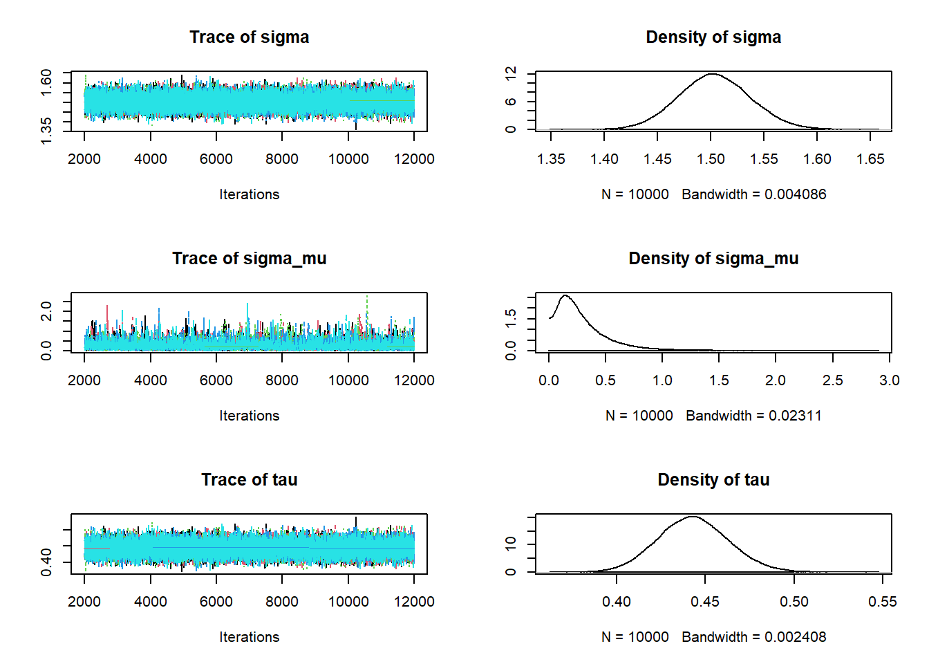
# data
data = read.csv("_data/baby_smoke.csv")

y = data$weight

x = (data$habit == "smoker") + 1

n = length(y)

n_groups = 2

# Model
model_string <- "model{

  # Likelihood
  for (i in 1:n){
  y[i] ~ dnorm(mu[x[i]], tau)
  }

  # Prior
  for (j in 1:n_groups){
  mu[j] ~ dnorm(mu0, 1 / sigma_mu ^ 2)
  }

  sigma <- 1 / sqrt(tau)
  tau ~ dgamma(1, 1)

  # Hyperprior
  mu0 ~ dnorm(7.5, 0.5)
  sigma_mu ~ dgamma(1, 3)

}"

dataList = list(y = y, x = x, n = n, n_groups = n_groups)

# Compile
model <- jags.model(textConnection(model_string),
                data = dataList,
                n.chains = 5)

## Compiling model graph
##    Resolving undeclared variables
##    Allocating nodes
## Graph information:
##    Observed stochastic nodes: 999
##    Unobserved stochastic nodes: 5
##    Total graph size: 2014
## 
## Initializing model

# Simulate
update(model, 1000, progress.bar = "none")

Nrep = 10000

posterior_sample <- coda.samples(model,
                             variable.names = c("mu", "tau", "sigma", "mu0", "sigma_mu"),
                             n.iter = Nrep,
                             progress.bar = "none")

# Summarize and check diagnostics
summary(posterior_sample)

## 
## Iterations = 2001:12000
## Thinning interval = 1 
## Number of chains = 5 
## Sample size per chain = 10000 
## 
## 1. Empirical mean and standard deviation for each variable,
##    plus standard error of the mean:
## 
##            Mean      SD   Naive SE Time-series SE
## mu[1]    7.1339 0.05120 0.00022896     0.00030865
## mu[2]    6.9050 0.13763 0.00061550     0.00138229
## mu0      7.0355 0.26165 0.00117013     0.00130730
## sigma    1.5035 0.03356 0.00015009     0.00015150
## sigma_mu 0.2898 0.24164 0.00108063     0.00370578
## tau      0.4430 0.01977 0.00008843     0.00008926
## 
## 2. Quantiles for each variable:
## 
##             2.5%    25%    50%    75%  97.5%
## mu[1]    7.03411 7.0991 7.1336 7.1684 7.2351
## mu[2]    6.62959 6.8105 6.9079 7.0057 7.1533
## mu0      6.49627 6.9189 7.0453 7.1447 7.5891
## sigma    1.43919 1.4807 1.5030 1.5259 1.5708
## sigma_mu 0.01636 0.1273 0.2266 0.3816 0.9273
## tau      0.40530 0.4295 0.4427 0.4561 0.4828

plot(posterior_sample)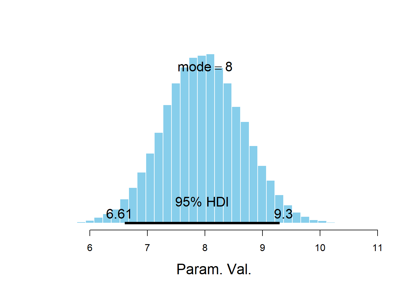

theta_sim_posterior = as.matrix(posterior_sample)
head(theta_sim_posterior)

##         mu[1]    mu[2]      mu0    sigma  sigma_mu       tau
## [1,] 7.118449 7.003762 7.056282 1.460830 0.2253755 0.4685985
## [2,] 7.186183 6.663398 6.928209 1.461622 0.2231579 0.4680904
## [3,] 7.145686 6.996485 7.266448 1.431581 0.2255716 0.4879416
## [4,] 7.168712 7.013768 7.045537 1.506650 0.2429123 0.4405299
## [5,] 7.134420 6.810429 7.060628 1.500137 0.1177805 0.4443634
## [6,] 7.123729 6.895591 6.849835 1.509891 0.2858626 0.4386406

theta_sim_posterior = as.data.frame(theta_sim_posterior)
names(theta_sim_posterior)[c(1, 2)] = c("mu1", "mu2")

ggplot(theta_sim_posterior, aes(mu1, mu2)) +
  geom_point(color = "skyblue", alpha = 0.4) +
  geom_density_2d(color = "orange", size = 1) +
  geom_abline(intercept = 0, slope = 1, color="black", 
             linetype="dashed")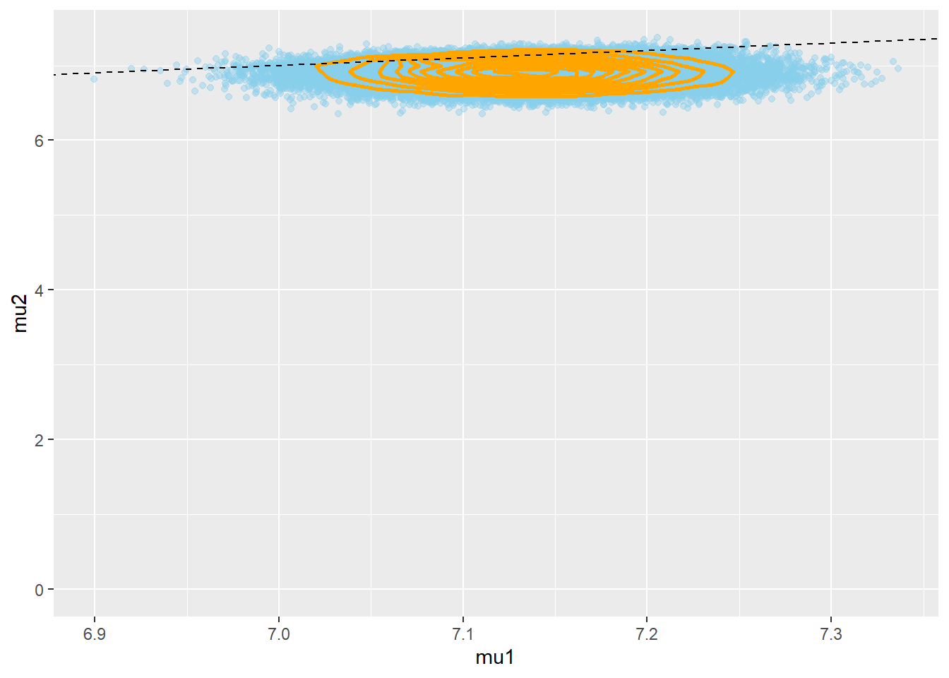

cor(theta_sim_posterior$mu1, theta_sim_posterior$mu2)

## [1] -0.02514047

mu_diff = theta_sim_posterior$mu1 - theta_sim_posterior$mu2

hist(mu_diff, xlab = "mu1 - mu2")
abline(v = quantile(mu_diff, c(0.025, 0.975)), lty = 2)

quantile(mu_diff, c(0.025, 0.975))

##        2.5%       97.5% 
## -0.02419377  0.52482421

mean(mu_diff)

## [1] 0.228875

sum(mu_diff > 0 ) / 50000

## [1] 0.94582

sigma = 1 / sqrt(theta_sim_posterior$tau)

effect_size = mu_diff / sigma

hist(effect_size, xlab = "effect size")
abline(v = quantile(effect_size, c(0.95)), lty = 2)

quantile(effect_size, c(0.95))

##       95% 
## 0.3187092

mean(effect_size)

## [1] 0.152358

The posterior distribution in the hierarchical model gives a little more credibility to a large difference in means. However, there are no major differences and the conclusions do not change substantially compared to those in 19.1.

I did test a few different priors for $\sigma_\mu$ and the other parameters, and the results are not very sensitive to choice of prior. For some discussion and recommendations regarding prior distributions for variance parameters, see Section 5.7 of Gelman et. al. Bayesian Data Analysis, 3rd ed.↩︎