6 Day 6 (June 12)
6.1 Announcements
Assignment 1 is graded
- General grading scheme
- General comments about reproducibility
- Too much computer code
- No or not enough computer code
- Computer code formatting (e.g., running over the page edge)
Questions about assignment 2
Live examples
6.2 Estimation
- Three options to estimate \(\boldsymbol{\beta}\)
- Minimize a loss function
- Maximize a likelihood function
- Find the posterior distribution
- Each option requires different assumptions
6.3 Loss function approach
- Define a measure of discrepancy between the data and the mathematical model
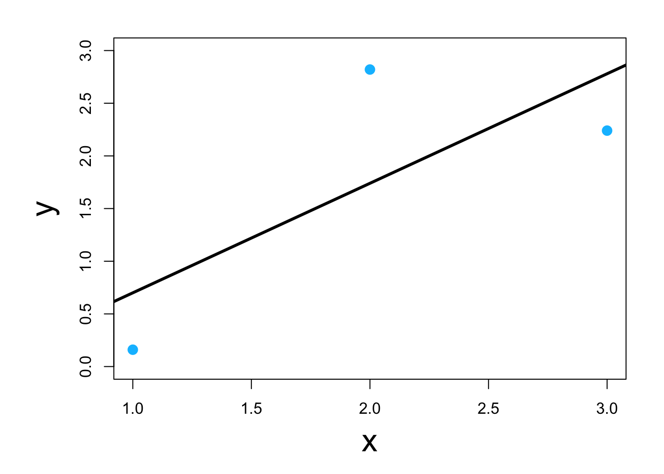
- Find the values of \(\boldsymbol{\beta}\) that make \(\mathbf{X}\boldsymbol{\beta}\) “closest” to \(\mathbf{y}\)
- Visual
- Classic example \[\underset{\boldsymbol{\beta}}{\operatorname{argmin}}\sum_{i=1}^{n}(y_i-\mathbf{x}_{i}^{\prime}\boldsymbol{\beta})^2\] or in matrix form \[\underset{\boldsymbol{\beta}}{\operatorname{argmin}}(\mathbf{y} - \mathbf{X}\boldsymbol{\beta})^{\prime}(\mathbf{y} - \mathbf{X}\boldsymbol{\beta})\] which results in \[\hat{\boldsymbol{\beta}}=(\mathbf{X}^{\prime}\mathbf{X})^{-1}\mathbf{X}^{\prime}\mathbf{y}\]
- Three ways to do it in program R
- Using scalar calculus and algebra (kind of)
y <- c(0.16,2.82,2.24)
x <- c(1,2,3)

y.bar <- mean(y)
x.bar <- mean(x)

# Estimate the slope parameter
beta1.hat <- sum((x-x.bar)*(y-y.bar))/sum((x-x.bar)^2)
beta1.hat
## [1] 1.04# Estimate the intercept parameter beta0.hat <- y.bar - sum((x-x.bar)*(y-y.bar))/sum((x-x.bar)^2)*x.bar beta0.hat## [1] -0.34- Using matrix calculus and algebra
y <- c(0.16,2.82,2.24)
X <- matrix(c(1,1,1,1,2,3),nrow=3,ncol=2,byrow=FALSE)
solve(t(X)%*%X)%*%t(X)%*%y
## [,1] ## [1,] -0.34 ## [2,] 1.04- Using modern (circa 1970’s) optimization techniques
y <- c(0.16,2.82,2.24)
x <- c(1,2,3)

optim(par=c(0,0),method = c("Nelder-Mead"),fn=function(beta){sum((y-(beta[1]+beta[2]*x))^2)})
## $par ## [1] -0.3399977 1.0399687 ## ## $value ## [1] 1.7496 ## ## $counts ## function gradient ## 61 NA ## ## $convergence ## [1] 0 ## ## $message ## NULL- Using modern and user friendly statistical computing software
df <- data.frame(y = c(0.16,2.82,2.24),x = c(1,2,3))
lm(y~x,data=df)
## ## Call: ## lm(formula = y ~ x, data = df) ## ## Coefficients: ## (Intercept) x ## -0.34 1.04 - Live example