26 Day 26 (July 12)
26.1 Announcements
- Work day on Thursday
- Guide and opportunity for improvement for assignment 3 is available
- Assignment 4 is posted and due next Friday
- Presentations will occur between Monday July 24 - Friday July 28.
- Please email me to request a 20-30 min time slot between 10:30 am and 4 pm to give your final presentation. When you email me, please give 3 dates/time that work for you.
- Read Ch. 6 (Model diagnostics) in Linear models with R
26.2 Distributional assumptions
Why did we assume \(\mathbf{y}\sim\text{N}(\mathbf{X\boldsymbol{\beta}},\sigma^{2}\mathbf{I})\)?
Is the assumption \(\mathbf{y}\sim\text{N}(\mathbf{X\boldsymbol{\beta}},\sigma^{2}\mathbf{I})\) ever correct? Is there a “true” model?
When would we expect the assumption \(\mathbf{y}\sim\text{N}(\mathbf{X\boldsymbol{\beta}},\sigma^{2}\mathbf{I})\) to be approximately correct?
- Human body weights
- Stock prices
- Temperature
- Proportion of votes for a candidate in an elections
Checking distributional assumptions
- If \(\mathbf{y}\sim\text{N}(\mathbf{X\boldsymbol{\beta}},\sigma^{2}\mathbf{I})\), then \(\mathbf{y} - \mathbf{X\boldsymbol{\beta}}\sim ?\)
If the assumption \(\mathbf{y}\sim\text{N}(\mathbf{X\boldsymbol{\beta}},\sigma^{2}\mathbf{I})\) is approximately correct, then what should \(\hat{\boldsymbol{\varepsilon}}\) look like?
Example: checking the assumption that \(\boldsymbol{\varepsilon}\sim\text{N}(\mathbf{0},\sigma^{2}\mathbf{I})\)
- Data
y <- c(63, 68, 61, 44, 103, 90, 107, 105, 76, 46, 60, 66, 58, 39, 64, 29, 37,
27, 38, 14, 38, 52, 84, 112, 112, 97, 131, 168, 70, 91, 52, 33, 33, 27,
18, 14, 5, 22, 31, 23, 14, 18, 23, 27, 44, 18, 19)
year <- 1965:2011
df <- data.frame(y = y, year = year)

plot(x = df$year, y = df$y, xlab = "Year", ylab = "Annual count", main = "",
col = "brown", pch = 20)
m1 <- lm(y ~ year, data = df)
abline(m1)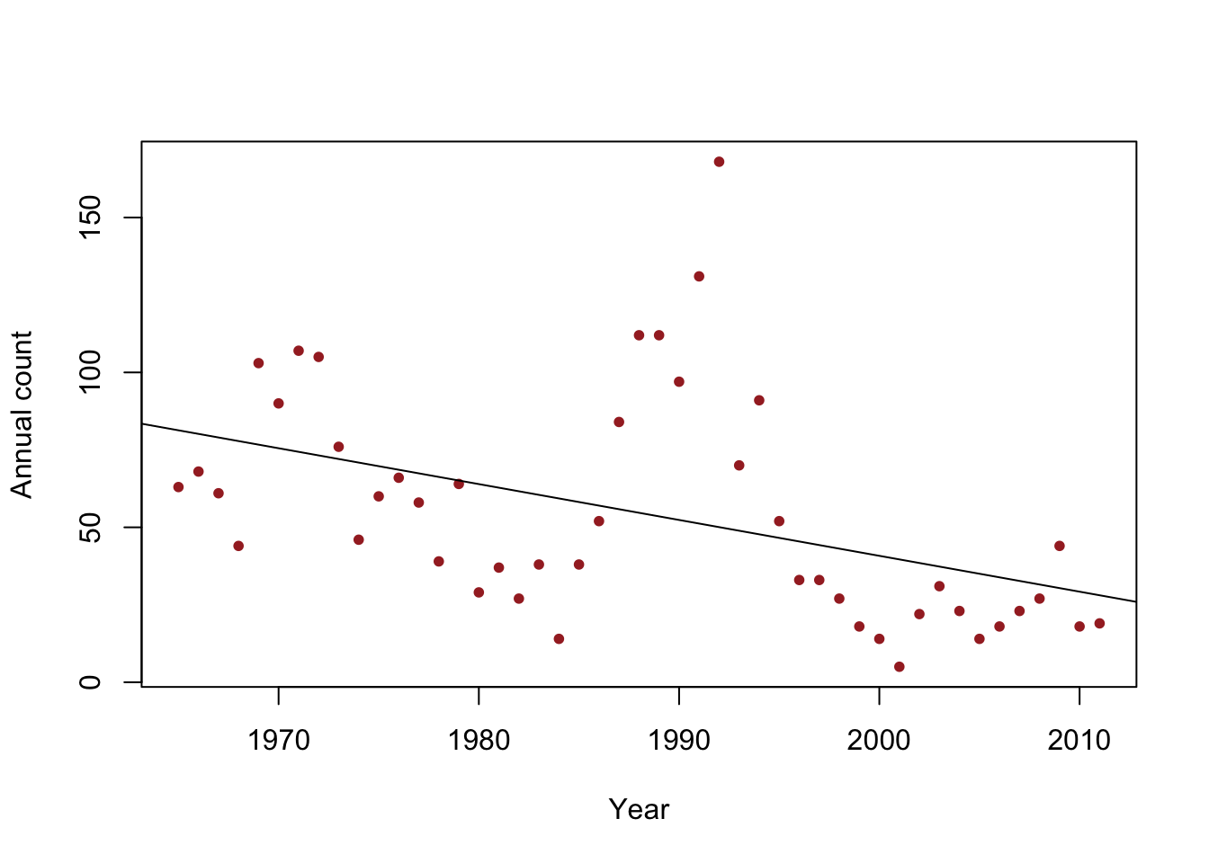
- Histogram of \(\hat{\boldsymbol{\varepsilon}}\)
m1 <- lm(y ~ year, data = df)
e.hat <- residuals(m1)
hist(e.hat,col="grey",breaks=15,main="",xlab=expression(hat(epsilon)))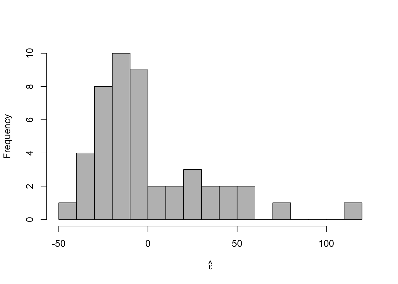
- Plot covariate vs. \(\hat{\boldsymbol{\varepsilon}}\)
plot(year,e.hat,xlab="Year",ylab=expression(hat(epsilon)),col="darkgreen")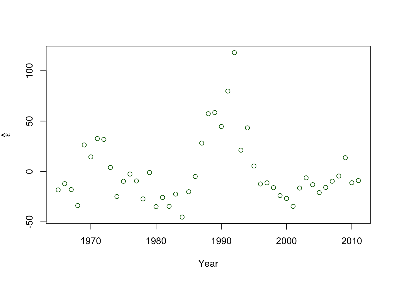
- A formal hypothesis test (see pg. 81 in Faraway (2014))
shapiro.test(e.hat)## ## Shapiro-Wilk normality test ## ## data: e.hat ## W = 0.86281, p-value = 5.709e-05Example: Checking the assumption that \(\boldsymbol{\varepsilon}\sim\text{N}\left(\mathbf{0},\sigma^{2}\mathbf{I}\right)\) (What it should look like)
- Simulated data
beta.truth <- c(2356,-1.15)
sigma2.truth <- 33^2
n <- 47


year <- 1965:2011
X <- model.matrix(~year)
set.seed(2930)
y <- rnorm(n,X%*%beta.truth,sigma2.truth^0.5)
df1 <- data.frame(y = y, year = year)

plot(x = df1$year, y = df1$y, xlab = "Year", ylab = "Annual count", main = "",
col = "brown", pch = 20)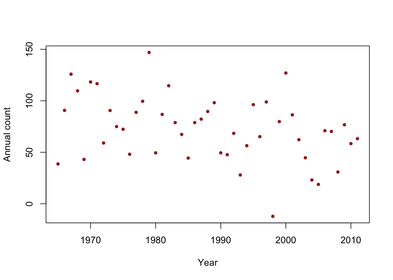
m2 <- lm(y ~ year,df1)
e.hat <- residuals(m2)

summary(m2)
## ## Call: ## lm(formula = y ~ year, data = df1) ## ## Residuals: ## Min 1Q Median 3Q Max ## -76.757 -22.237 3.767 19.353 66.634 ## ## Coefficients: ## Estimate Std. Error t value Pr(>|t|) ## (Intercept) 1717.2121 638.5293 2.689 0.0100 * ## year -0.8272 0.3212 -2.575 0.0134 * ## --- ## Signif. codes: 0 '***' 0.001 '**' 0.01 '*' 0.05 '.' 0.1 ' ' 1 ## ## Residual standard error: 29.87 on 45 degrees of freedom ## Multiple R-squared: 0.1285, Adjusted R-squared: 0.1091 ## F-statistic: 6.632 on 1 and 45 DF, p-value: 0.01337- Histogram of \(\hat{\boldsymbol{\varepsilon}}\)
hist(e.hat,col="grey",breaks=15,main="",xlab=expression(hat(epsilon)))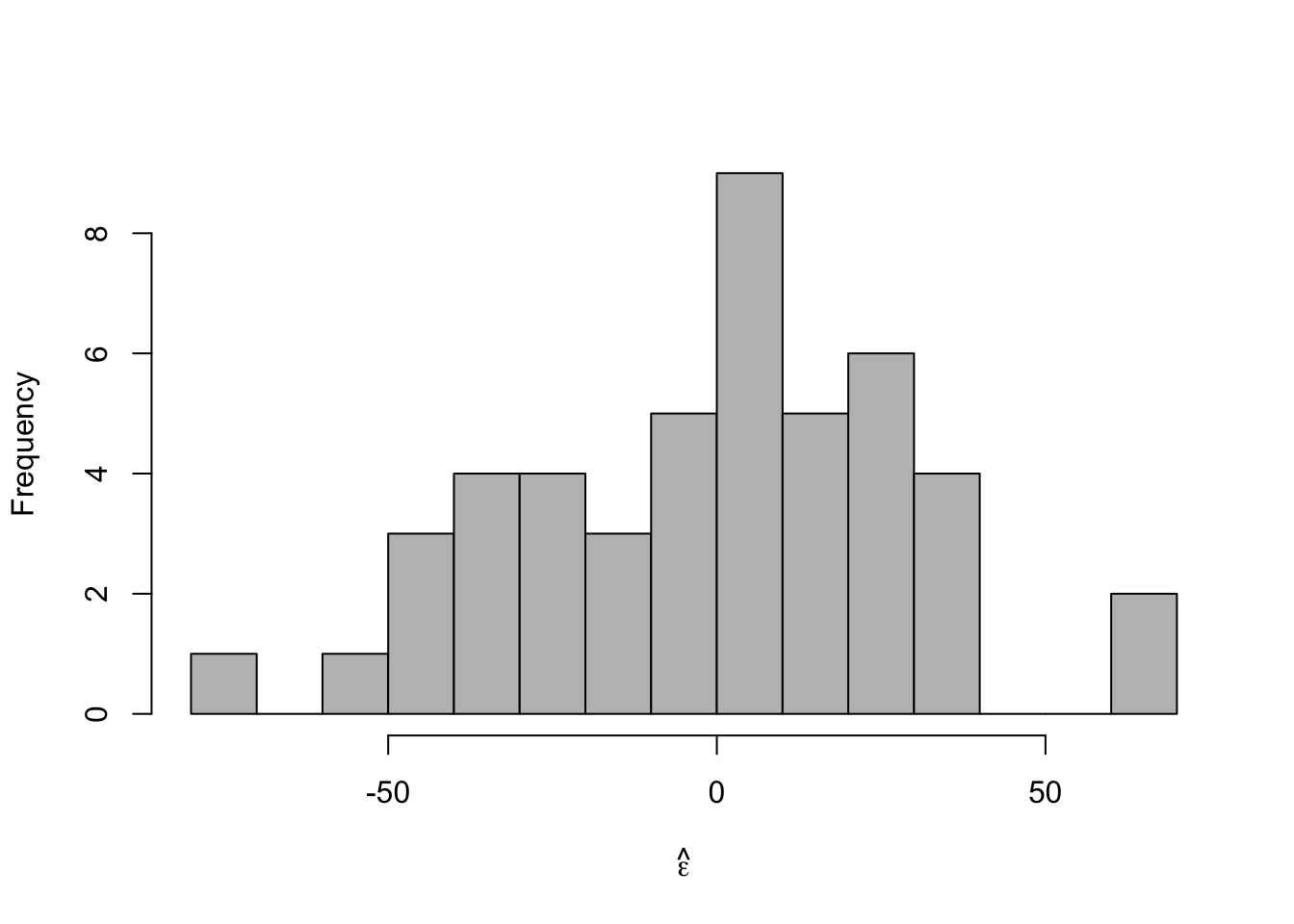
- Plot covariate vs. \(\hat{\boldsymbol{\varepsilon}}\)
plot(year,e.hat,xlab="Year",ylab=expression(hat(epsilon)))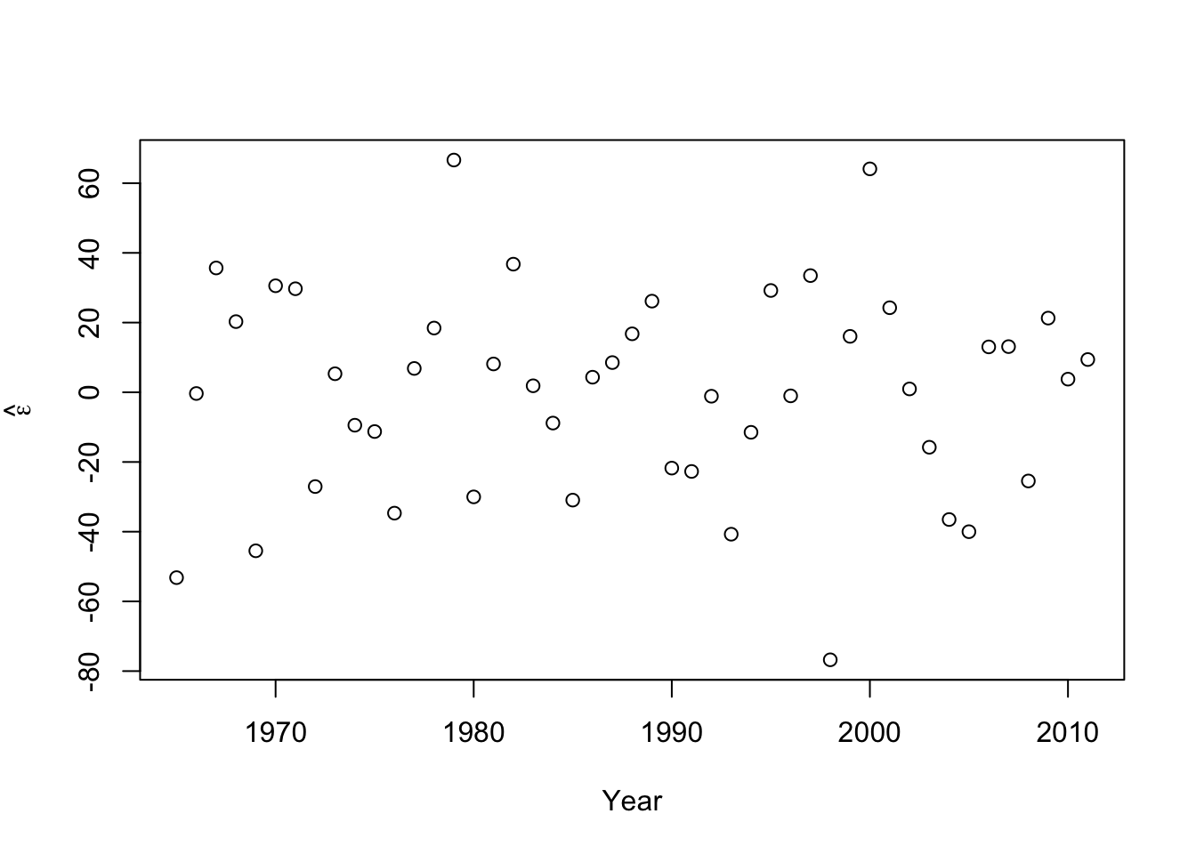
- A formal hypothesis test (see pg. 81 in Faraway (2014))
shapiro.test(e.hat)## ## Shapiro-Wilk normality test ## ## data: e.hat ## W = 0.98556, p-value = 0.8228
26.3 Constant variance
If \(\mathbf{y}\sim\text{N}(\mathbf{X\boldsymbol{\beta}},\sigma^{2}\mathbf{I})\), then each \(\varepsilon_i\) follows a normal distribution with the same value of \(\sigma^2\).
- A linear model with constant variance is the simplest possible model we could assume. It is like the intercept only model in that regard.
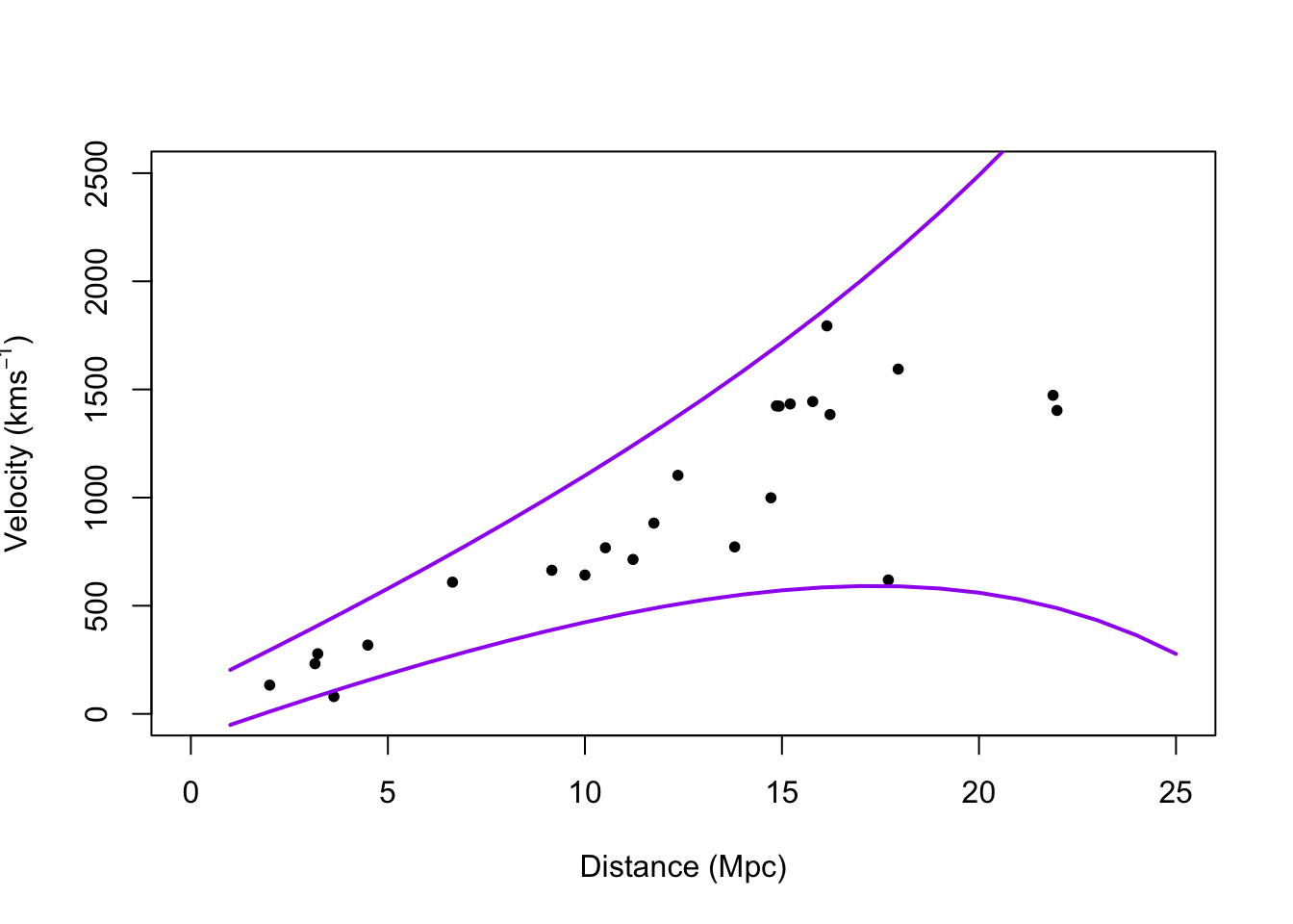
- Example: Hubble data
library(gamair)
data(hubble)

m1 <- lm(y ~ x - 1, data = hubble)
confint(m1)
## 2.5 % 97.5 % ## x 68.37937 84.78297# Plot data and E(y) plot(hubble$x,hubble$y,xlab="Distance (Mpc)", ylab=expression("Velocity (km"*s^{-1}*")"),pch=20) abline(m1)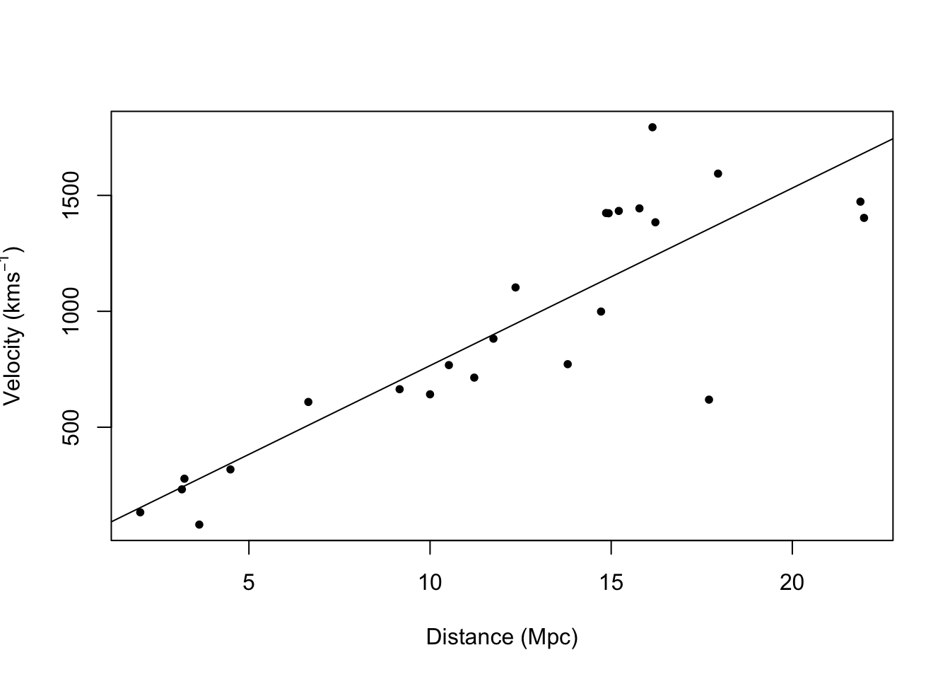
# Plot residuals vs. x
e.hat <- residuals(m1)
hist(e.hat,col="grey",breaks=15,main="",xlab=expression(hat(epsilon)))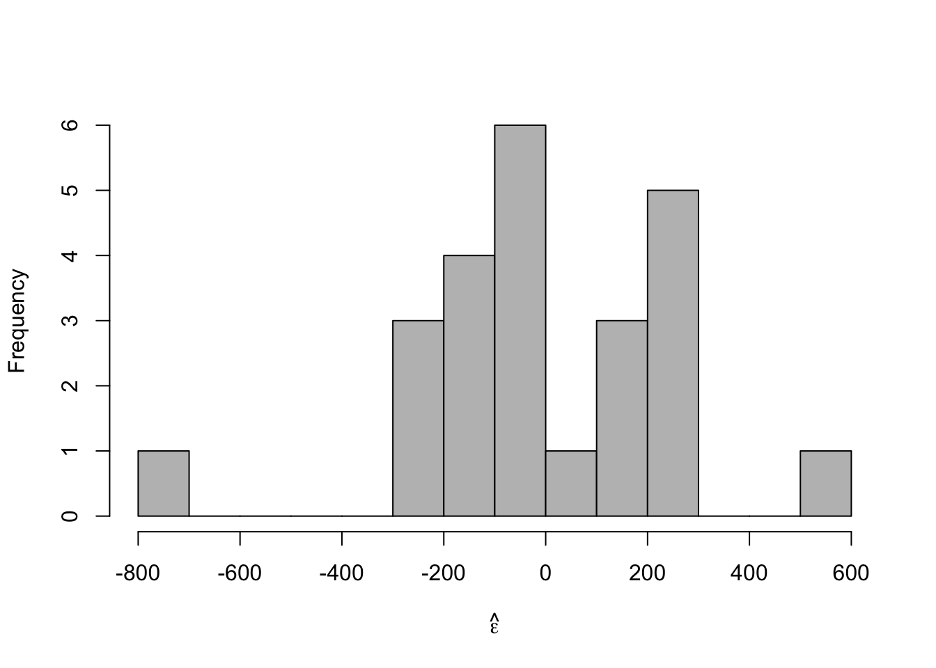
plot(hubble$x,e.hat,xlab="Distance(Mpc)",ylab=expression(hat(epsilon)),pch=20)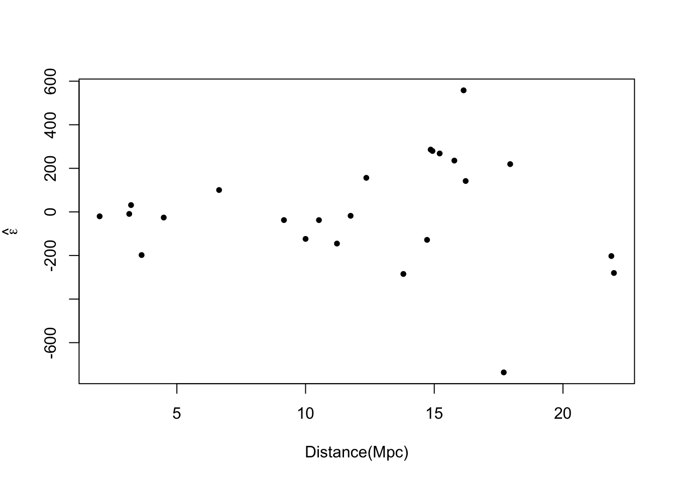
# Plot prediction intervals
y.pi <- predict(m1,newdata=data.frame(x = 0:25),interval = "predict")
plot(hubble$x,hubble$y,xlab="Distance (Mpc)",
ylab=expression("Velocity (km"*s^{-1}*")"),xlim=c(0,25),ylim=c(0,2500),pch=20)
points(0:25,y.pi[,2],typ="l",lwd=2,col="purple")
points(0:25,y.pi[,3],typ="l",lwd=2,col="purple")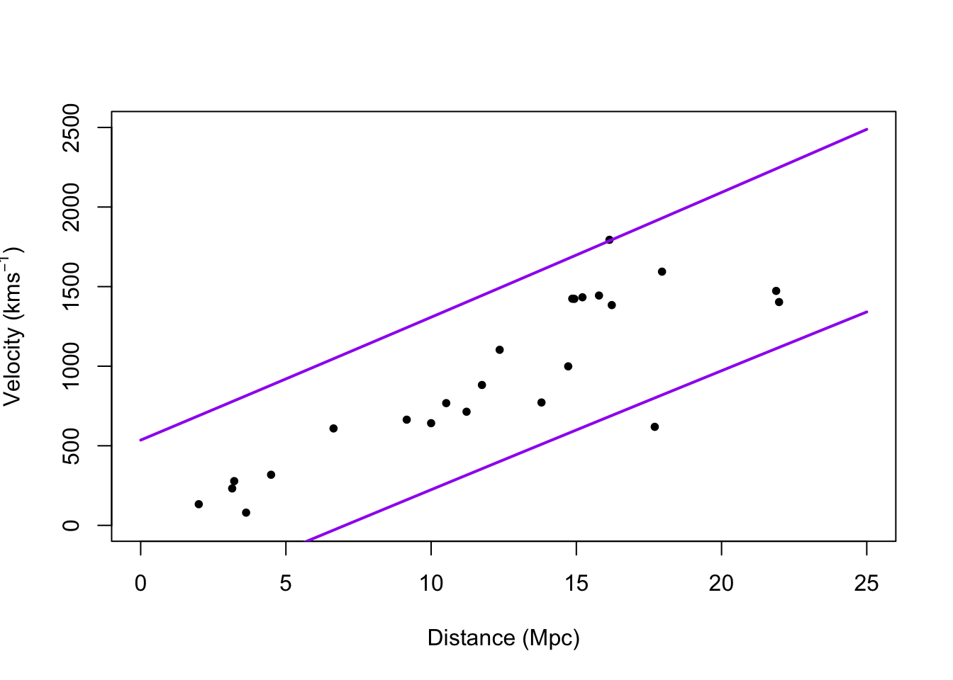
- A test for equal variance (see pg. 77 in Faraway (2014))
- What causes non-constant variance (also called heteroskedasticity).
What can be done?
- A transformation may work (see pg. 77 Faraway (2014))
- Build a more appropriate model for the variance. For example, \[\mathbf{y}\sim\text{N}(\mathbf{X\boldsymbol{\beta}},\mathbf{V})\] where the \(i^\text{th}\) and \(j^{th}\) entry of the matrix \(\mathbf{V}\) equals \[v_{ij}(\theta)=\begin{cases} \sigma^{2}e^{2\theta x_i} &\text{if}\ i=j\\ 0 &\text{if}\ i\neq j \end{cases}\]
library(nlme)
m2 <- gls(y~x-1,weights = varExp(form=~x),data=hubble)
summary(m2)
## Generalized least squares fit by REML ## Model: y ~ x - 1 ## Data: hubble ## AIC BIC logLik ## 322.432 325.8385 -158.216 ## ## Variance function: ## Structure: Exponential of variance covariate ## Formula: ~x ## Parameter estimates: ## expon ## 0.1060336 ## ## Coefficients: ## Value Std.Error t-value p-value ## x 76.2548 3.854585 19.78288 0 ## ## Standardized residuals: ## Min Q1 Med Q3 Max ## -2.4272668 -0.4726915 -0.1548023 0.7929118 1.8437320 ## ## Residual standard error: 55.17695 ## Degrees of freedom: 24 total; 23 residualconfint(m2)## 2.5 % 97.5 % ## x 68.69995 83.80965# Plot prediction intervals X <- model.matrix(y~x-1,data=hubble) sigma2.hat <- summary(m1)$sigma^2 sigma2.hat*solve(t(X)%*%X)## x ## x 15.71959vcov(m1)## x ## x 15.71959X <- model.matrix(y~x-1,data=hubble) beta.hat <- coef(m2) sigma2.hat <- summary(m2)$sigma^2 theta.hat <- summary(m2)$modelStruct$varStruct V <- diag(c(sigma2.hat*exp(2*X%*%theta.hat))) X.new <- model.matrix(~x-1,data=data.frame(x = 1:25)) y.pi <- cbind(X.new%*%beta.hat - qt(0.975,24-1)*sqrt(X.new^2%*%solve(t(X)%*%solve(V)%*%X) + sigma2.hat*exp(2*X.new%*%theta.hat)), X.new%*%beta.hat + qt(0.975,24-1)*sqrt(X.new^2%*%solve(t(X)%*%solve(V)%*%X) + sigma2.hat*exp(2*X.new%*%theta.hat))) plot(hubble$x,hubble$y,xlab="Distance (Mpc)", ylab=expression("Velocity (km"*s^{-1}*")"),xlim=c(0,25),ylim=c(0,2500),pch=20) points(1:25,y.pi[,1],typ="l",lwd=2,col="purple") points(1:25,y.pi[,2],typ="l",lwd=2,col="purple")