34 Day 34 (July 24)
34.1 Announcements
Presentations will be in this room unless otherwise noted (e.g., in my email I probably said go do Dickens 109).
Get peer reviews in this week!
Up next
- Random effects/mixed model
- Generalized linear models
- Machine learning (e.g., regression trees, random forest)
- Generalized additive models
34.2 Random effects
Conditional, marginal, and joint distributions
- Conditional distribution: “\(\mathbf{y}\) given \(\boldsymbol{\beta}\)” \[\mathbf{y}|\boldsymbol{\beta}\sim\text{N}(\mathbf{X}\boldsymbol{\beta},\sigma_{\varepsilon}^{2}\mathbf{I})\] This is also sometimes called the data model.
- Marginal distribution of \(\boldsymbol{\beta}\) \[\beta\sim\text{N}(\mathbf{0},\sigma_{\beta}^{2}\mathbf{I})\] This is also called the parameter model.
- Joint distribution \([\mathbf{y}|\boldsymbol{\beta}][\boldsymbol{\beta}]\)
Estimation for the linear model with random effects
- By maximizing the joint likelihood
- Write out the likelihood function \[\mathcal{L}(\boldsymbol{\beta},\sigma_{\varepsilon},\sigma_{\beta}^{2})=\frac{1}{(2\pi)^{-\frac{n}{2}}}|\sigma^{2}_{\varepsilon}\mathbf{I}|^{-\frac{1}{2}}\text{exp}\bigg{(}-\frac{1}{2}(\mathbf{y} - \mathbf{X}\boldsymbol{\beta})^{\prime}(\sigma^{2}_{\varepsilon}\mathbf{I})^{-1}(\mathbf{y} - \mathbf{X}\boldsymbol{\beta})\bigg{)}\times\\\frac{1}{(2\pi)^{-\frac{p}{2}}}|\sigma^{2}_{\beta}\mathbf{I}|^{-\frac{1}{2}}\text{exp}\bigg{(}-\frac{1}{2}\boldsymbol{\beta}^{\prime}(\sigma^{2}_{\beta}\mathbf{I})^{-1}\boldsymbol{\beta}\bigg{)}\]
- Maximizing the log-likelihood function w.r.t. gives \(\boldsymbol{\beta}\) gives \[\hat{\boldsymbol{\beta}}=\big{(}\mathbf{X}^{'}\mathbf{X}+\frac{\sigma^{2}_{\varepsilon}}{\sigma^{2}_{\beta}}\mathbf{I}\big{)}^{-1}\mathbf{X}^{'}\mathbf{y}\]
- By maximizing the joint likelihood
Example eye temperature data set for Eurasian blue tit
df.et <- read.table("https://www.dropbox.com/s/bo11n66cezdnbia/eyetemp.txt?dl=1")
names(df.et) <- c("id","sex","date","time","event","airtemp","relhum","sun","bodycond","eyetemp")
df.et$id <- as.factor(df.et$id)
df.et$id.num <- as.numeric(df.et$id)

ind.means <- aggregate(eyetemp ~ id.num,df.et, FUN=base::mean)
plot(df.et$id.num,df.et$eyetemp,xlab="Individual",ylab="Eye temperature")
points(ind.means,pch="x",col="gold",cex=1.5)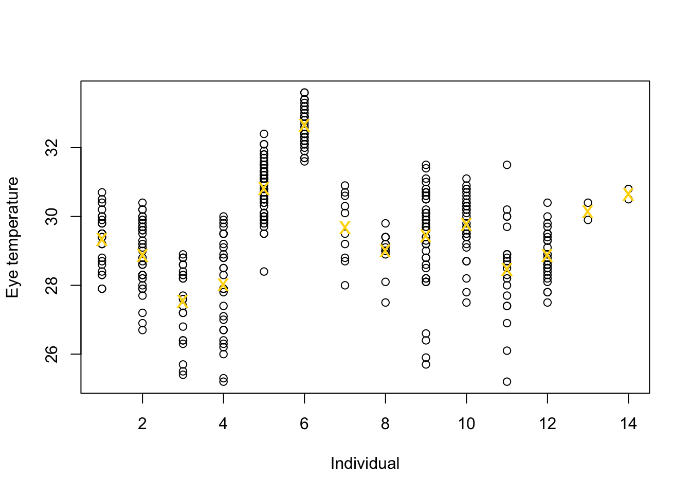
# Standard "fixed effects" linear regression model
m1 <- lm(eyetemp~as.factor(id.num)-1,data=df.et)
summary(m1)
## ## Call: ## lm(formula = eyetemp ~ as.factor(id.num) - 1, data = df.et) ## ## Residuals: ## Min 1Q Median 3Q Max ## -3.7378 -0.5750 0.1507 0.6622 3.0286 ## ## Coefficients: ## Estimate Std. Error t value Pr(>|t|) ## as.factor(id.num)1 29.3423 0.1972 148.77 <2e-16 *** ## as.factor(id.num)2 28.8735 0.1725 167.41 <2e-16 *** ## as.factor(id.num)3 27.5458 0.2053 134.19 <2e-16 *** ## as.factor(id.num)4 28.0156 0.1778 157.59 <2e-16 *** ## as.factor(id.num)5 30.8188 0.1211 254.56 <2e-16 *** ## as.factor(id.num)6 32.6486 0.1700 192.06 <2e-16 *** ## as.factor(id.num)7 29.6800 0.3180 93.33 <2e-16 *** ## as.factor(id.num)8 29.0000 0.2789 103.97 <2e-16 *** ## as.factor(id.num)9 29.4378 0.1499 196.36 <2e-16 *** ## as.factor(id.num)10 29.7667 0.1836 162.12 <2e-16 *** ## as.factor(id.num)11 28.4714 0.2195 129.74 <2e-16 *** ## as.factor(id.num)12 28.8793 0.1867 154.64 <2e-16 *** ## as.factor(id.num)13 30.1500 0.7111 42.40 <2e-16 *** ## as.factor(id.num)14 30.6500 0.7111 43.10 <2e-16 *** ## --- ## Signif. codes: 0 '***' 0.001 '**' 0.01 '*' 0.05 '.' 0.1 ' ' 1 ## ## Residual standard error: 1.006 on 358 degrees of freedom ## Multiple R-squared: 0.9989, Adjusted R-squared: 0.9989 ## F-statistic: 2.31e+04 on 14 and 358 DF, p-value: < 2.2e-16plot(df.et$id.num,df.et$eyetemp,xlab="Individual",ylab="Expected eye temperature",col="white") points(1:14,coef(m1),pch=20,col="black",cex=1) segments (1:14,confint(m1)[,1],1:14,confint(m1)[,2] ,lwd=2,lty=1)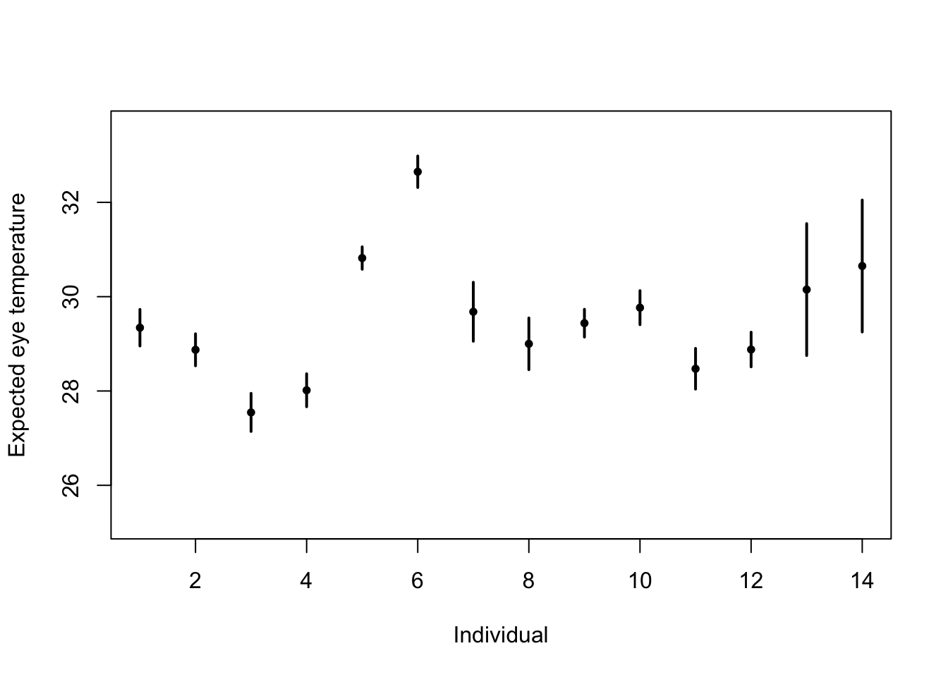
# Random effects regression model (using nlme package; difficult to get confidence interval)
library(nlme)
m2 <- lme(fixed = eyetemp ~ 1,random= list(id = pdIdent(~id-1)),data=df.et,method="ML")#summary(m2)
#predict(m2,level=1,newdata=data.frame(id=unique(df.et$id)))

# Random effects regression model (mgcv package)
library(mgcv)
m2 <- gam(eyetemp ~ 1+s(id,bs="re"),data=df.et,method="ML")

plot(df.et$id.num,df.et$eyetemp,xlab="Individual",ylab="Expected eye temperature",col="white")
points(1:14-0.15,coef(m1),pch=20,col="black",cex=1)
segments (1:14-0.15,confint(m1)[,1],1:14-0.15,confint(m1)[,2] ,lwd=2,lty=1)
pred <- predict(m2,newdata=data.frame(id=unique(df.et$id)),se.fit=TRUE)
pred$lci <- pred$fit - 1.96*pred$se.fit
pred$uci <- pred$fit + 1.96*pred$se.fit
points(1:14+0.15,pred$fit,pch=20,col="green",cex=1)
segments (1:14+0.15,pred$lci,1:14+0.15,pred$uci,lwd=2,lty=1,col="green")
abline(a=coef(m2)[1],b=0,col="grey")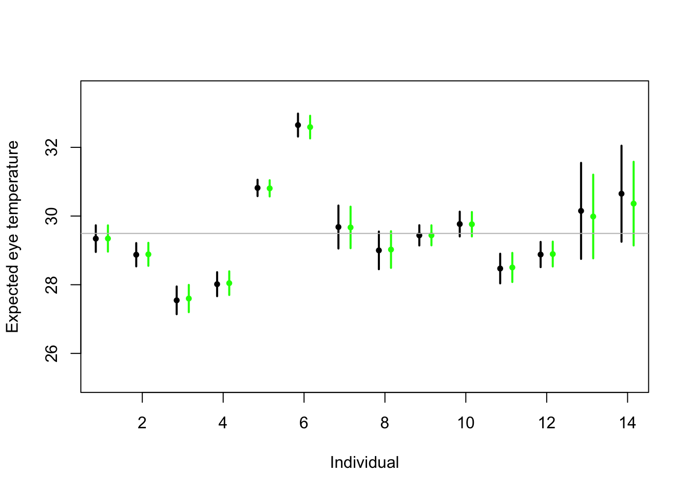
Summary
- Take home message
- Treating \(\boldsymbol{\beta}\) as a random effect “shrinks” the estimates of \(\boldsymbol{\beta}\) closer to zero.
- Requires an extra assumption \(\boldsymbol{\beta}\sim\text{N}(\mathbf{0},\sigma_{\beta}^{2}\mathbf{I})\)
- Penalty
- Random effect
- This called a prior distribution in Bayesian statistics
- Take home message