11 Day 11 (June 19)
11.3 Confidence intervals for paramters
Example
y <- c(63, 68, 61, 44, 103, 90, 107, 105, 76, 46, 60, 66, 58, 39, 64, 29, 37,
27, 38, 14, 38, 52, 84, 112, 112, 97, 131, 168, 70, 91, 52, 33, 33, 27,
18, 14, 5, 22, 31, 23, 14, 18, 23, 27, 44, 18, 19)
year <- 1965:2011
df <- data.frame(y = y, year = year)
plot(x = df$year, y = df$y, xlab = "Year", ylab = "Annual count", main = "",
col = "brown", pch = 20, xlim = c(1965, 2040))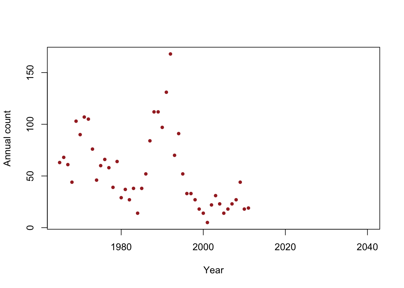
- Is the population size really decreasing?
- Write out the model we should use answer this question
- How can we assess the uncertainty in our estimate of \(\beta_1\)?
- Confidence intervals in R
m1 <- lm(y~year,data=df)
coef(m1)
## (Intercept) year ## 2356.48797 -1.15784confint(m1,level=0.95)## 2.5 % 97.5 % ## (Intercept) 929.80699 3783.1689540 ## year -1.87547 -0.4402103- Note \[\hat{\boldsymbol{\beta}}\sim\text{N}(\boldsymbol{\beta},\sigma^2(\mathbf{X}^{\prime}\mathbf{X})^{-1})\] and let \[\hat{\beta_1}\sim\text{N}(\beta_1,\sigma^{2}_{\beta_1})\] where \(\sigma^{2}_{\beta_1}= \sigma^2\mathbf{c}^{\prime}(\mathbf{X}^{\prime}\mathbf{X})^{-1}\mathbf{c}\) and \(\mathbf{c}\equiv(0,1,0,0,\ldots,0)^{\prime}\). In R we can extract \(\sigma^2(\mathbf{X}^{\prime}\mathbf{X})^{-1}\) using
vcov().
vcov(m1)## (Intercept) year ## (Intercept) 501753.2825 -252.3792372 ## year -252.3792 0.1269513Note that
diag(vcov(m1))^0.5## (Intercept) year ## 708.3454542 0.3563023corresponds to the column
Std. Errorfromsummary()summary(m1)## ## Call: ## lm(formula = y ~ year, data = df) ## ## Residuals: ## Min 1Q Median 3Q Max ## -45.333 -20.597 -9.754 14.035 117.929 ## ## Coefficients: ## Estimate Std. Error t value Pr(>|t|) ## (Intercept) 2356.4880 708.3455 3.327 0.00176 ** ## year -1.1578 0.3563 -3.250 0.00219 ** ## --- ## Signif. codes: 0 '***' 0.001 '**' 0.01 '*' 0.05 '.' 0.1 ' ' 1 ## ## Residual standard error: 33.13 on 45 degrees of freedom ## Multiple R-squared: 0.1901, Adjusted R-squared: 0.1721 ## F-statistic: 10.56 on 1 and 45 DF, p-value: 0.00219- When \(\sigma_{\beta_1}\) is known \[\hat{\beta_1}\sim\text{N}(\beta_1,\sigma^{2}_{\beta_1})\] \[\hat{\beta_1} - \beta_1 \sim\text{N}(0,\sigma^{2}_{\beta_1})\] \[\frac{\hat{\beta_1} - \beta_1}{\sigma_{\beta_1}} \sim\text{N}(0,1)\]
- When \(\sigma_{\beta_1}\) is estimated \[\frac{\hat{\beta_1} - \beta_1}{\hat{\sigma}_{\beta_1}} \sim\text{t}(\nu)\] where \(\nu = n - p\)
- Deriving the confidence interval for \(\hat{\beta_1}\) \[\text{P}(a < \frac{\hat{\beta_1} - \beta_1}{\hat{\sigma}_{\beta_1}} < b) = 1-\alpha\] \[\text{P}(a\hat{\sigma}_{\beta_1} < \hat{\beta_1} - \beta_1 < b\hat{\sigma}_{\beta_1}) = 1-\alpha\] \[\text{P}(-\hat{\beta_1} + a\hat{\sigma}_{\beta_1} < - \beta_1 < -\hat{\beta_1} + b\hat{\sigma}_{\beta_1}) = 1-\alpha\] \[\text{P}(\hat{\beta_1} - b\hat{\sigma}_{\beta_1} < \beta_1 < \hat{\beta_1} - a\hat{\sigma}_{\beta_1}) = 1-\alpha\]
- What is \(\text{P}(a < \frac{\hat{\beta_1} - \beta_1}{\hat{\sigma}_{\beta_1}} < b) = 1-\alpha\)? \[\text{P}(a < z < b) = \int_{a}^{b}[z|\nu]dz\]
- “By hand” in R
nu <- length(df$y) - 2
a <- qt(p = 0.025,df = nu)
a
## [1] -2.014103b <- qt(p = 0.975,df = nu) b## [1] 2.014103beta1.hat <- coef(m1)[2] sigma.beta1.hat <- (diag(vcov(m1))^0.5)[2] beta1.hat - b*sigma.beta1.hat## year ## -1.87547beta1.hat - a*sigma.beta1.hat## year ## -0.4402103confint(m1)[2,]## 2.5 % 97.5 % ## -1.8754696 -0.4402103