12 Day 12 (June 20)
12.1 Announcements
- Assignment 2 is graded
- Guide is available
- Learning opportunities
- Questions about assignment 3?
12.2 Confidence intervals for paramters
Example
y <- c(63, 68, 61, 44, 103, 90, 107, 105, 76, 46, 60, 66, 58, 39, 64, 29, 37,
27, 38, 14, 38, 52, 84, 112, 112, 97, 131, 168, 70, 91, 52, 33, 33, 27,
18, 14, 5, 22, 31, 23, 14, 18, 23, 27, 44, 18, 19)
year <- 1965:2011
df <- data.frame(y = y, year = year)
plot(x = df$year, y = df$y, xlab = "Year", ylab = "Annual count", main = "",
col = "brown", pch = 20, xlim = c(1965, 2040))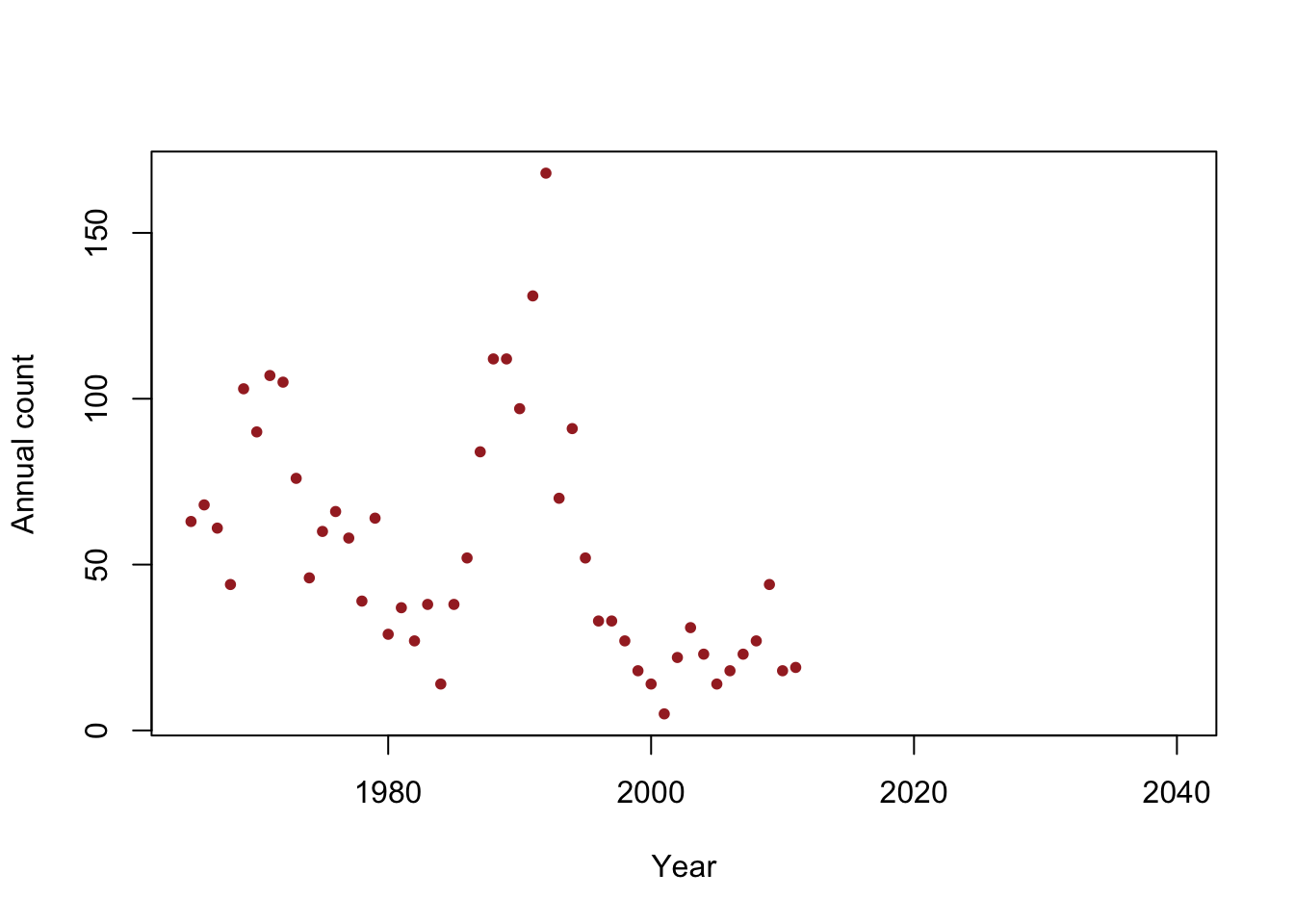
- Is the population size really decreasing?
- Write out the model we should use answer this question
- How can we assess the uncertainty in our estimate of \(\beta_1\)?
- Confidence intervals in R
m1 <- lm(y~year,data=df)
coef(m1)
## (Intercept) year ## 2356.48797 -1.15784confint(m1,level=0.95)## 2.5 % 97.5 % ## (Intercept) 929.80699 3783.1689540 ## year -1.87547 -0.4402103- Note \[\hat{\boldsymbol{\beta}}\sim\text{N}(\boldsymbol{\beta},\sigma^2(\mathbf{X}^{\prime}\mathbf{X})^{-1})\] and let \[\hat{\beta_1}\sim\text{N}(\beta_1,\sigma^{2}_{\beta_1})\] where \(\sigma^{2}_{\beta_1}= \sigma^2\mathbf{c}^{\prime}(\mathbf{X}^{\prime}\mathbf{X})^{-1}\mathbf{c}\) and \(\mathbf{c}\equiv(0,1,0,0,\ldots,0)^{\prime}\). In R we can extract \(\sigma^2(\mathbf{X}^{\prime}\mathbf{X})^{-1}\) using
vcov().
vcov(m1)## (Intercept) year ## (Intercept) 501753.2825 -252.3792372 ## year -252.3792 0.1269513Note that
diag(vcov(m1))^0.5## (Intercept) year ## 708.3454542 0.3563023corresponds to the column
Std. Errorfromsummary()summary(m1)## ## Call: ## lm(formula = y ~ year, data = df) ## ## Residuals: ## Min 1Q Median 3Q Max ## -45.333 -20.597 -9.754 14.035 117.929 ## ## Coefficients: ## Estimate Std. Error t value Pr(>|t|) ## (Intercept) 2356.4880 708.3455 3.327 0.00176 ** ## year -1.1578 0.3563 -3.250 0.00219 ** ## --- ## Signif. codes: 0 '***' 0.001 '**' 0.01 '*' 0.05 '.' 0.1 ' ' 1 ## ## Residual standard error: 33.13 on 45 degrees of freedom ## Multiple R-squared: 0.1901, Adjusted R-squared: 0.1721 ## F-statistic: 10.56 on 1 and 45 DF, p-value: 0.00219- When \(\sigma_{\beta_1}\) is known \[\hat{\beta_1}\sim\text{N}(\beta_1,\sigma^{2}_{\beta_1})\] \[\hat{\beta_1} - \beta_1 \sim\text{N}(0,\sigma^{2}_{\beta_1})\] \[\frac{\hat{\beta_1} - \beta_1}{\sigma_{\beta_1}} \sim\text{N}(0,1)\]
- When \(\sigma_{\beta_1}\) is estimated \[\frac{\hat{\beta_1} - \beta_1}{\hat{\sigma}_{\beta_1}} \sim\text{t}(\nu)\] where \(\nu = n - p\)
- Deriving the confidence interval for \(\hat{\beta_1}\) \[\text{P}(a < \frac{\hat{\beta_1} - \beta_1}{\hat{\sigma}_{\beta_1}} < b) = 1-\alpha\] \[\text{P}(a\hat{\sigma}_{\beta_1} < \hat{\beta_1} - \beta_1 < b\hat{\sigma}_{\beta_1}) = 1-\alpha\] \[\text{P}(-\hat{\beta_1} + a\hat{\sigma}_{\beta_1} < - \beta_1 < -\hat{\beta_1} + b\hat{\sigma}_{\beta_1}) = 1-\alpha\] \[\text{P}(\hat{\beta_1} - b\hat{\sigma}_{\beta_1} < \beta_1 < \hat{\beta_1} - a\hat{\sigma}_{\beta_1}) = 1-\alpha\]
- What is \(\text{P}(a < \frac{\hat{\beta_1} - \beta_1}{\hat{\sigma}_{\beta_1}} < b) = 1-\alpha\)? \[\text{P}(a < z < b) = \int_{a}^{b}[z|\nu]dz\]
- “By hand” in R
nu <- length(df$y) - 2
a <- qt(p = 0.025,df = nu)
a
## [1] -2.014103b <- qt(p = 0.975,df = nu) b## [1] 2.014103beta1.hat <- coef(m1)[2] sigma.beta1.hat <- (diag(vcov(m1))^0.5)[2] beta1.hat - b*sigma.beta1.hat## year ## -1.87547beta1.hat - a*sigma.beta1.hat## year ## -0.4402103confint(m1)[2,]## 2.5 % 97.5 % ## -1.8754696 -0.4402103
12.3 Monte Carlo simulation
Numerical method that allows us to play “what if” scenarios
- Using a single synthetic data set vs. multiple synthetic data sets
- Explore properties for realistic sample sizes
For Loops in R
for(i in 1:10){
  print(i)
}
## [1] 1 ## [1] 2 ## [1] 3 ## [1] 4 ## [1] 5 ## [1] 6 ## [1] 7 ## [1] 8 ## [1] 9 ## [1] 10Example
library(latex2exp)
library(nlme)
## ## Attaching package: 'nlme'## The following object is masked from 'package:dplyr': ## ## collapsebeta.truth <- c(3,1) # True value of beta sigma2.truth <- 1000 # True value of sigma2 q.sims <- 10^3 # How many data sets should I simulate? n <- 10 # Sample size for each simulated data set x <- seq(0,100,length.out = n) # Covariate X <- model.matrix (~x) # Design matrix sim.results <- matrix(,nrow=q.sims,ncol=2) colnames(sim.results) <- c("sigma2.reml","sigma2.ml") set.seed(4359) for(i in 1:q.sims){ y <- X%*%beta.truth + rnorm(n,0,sqrt(sigma2.truth)) # Generate data m1 <- gls(y~x,method="ML") m2 <- gls(y~x,method="REML") sim.results[i,1:2] <- c(summary(m1)$sigma^2,summary(m2)$sigma^2) } # Mean of sigma2 mean(sim.results[,1])## [1] 815.1985mean(sim.results[,2])## [1] 1018.998# Histogram of sigma2 par(mfrow=c(1,2)) hist(sim.results[,1],col="grey",xlab=TeX('$$\\hat{$\\sigma}^{2}'),main="ML") abline(v=sigma2.truth,col="gold",lwd=3) abline(v=mean(sim.results[,1]),col="red",lwd=3,lty=2) hist(sim.results[,2],col="grey",xlab=TeX('$$\\hat{$\\sigma}^{2}'),main="REML") abline(v=sigma2.truth,col="gold",lwd=3) abline(v=mean(sim.results[,2]),col="red",lwd=3,lty=2)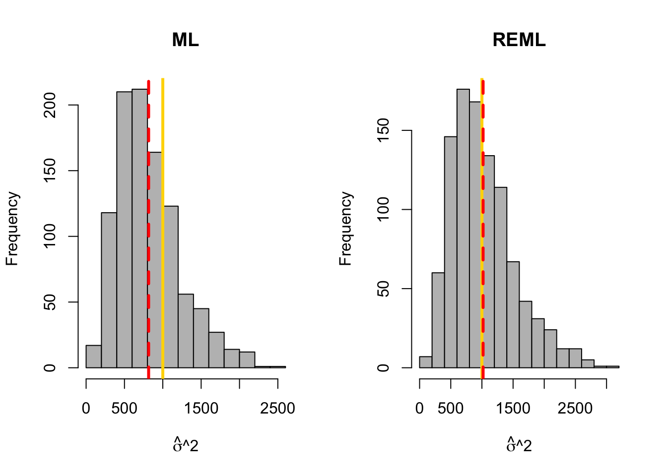
12.4 Understanding confidence intervals using synthetic data
What should we expect from a confidence interval?
- What is the statistic?
- Which quantities are random and which are fixed?
- How often should a 95% CI covers the true value of \(\beta\)?
How do we know if a CI performs as advertised?
- Derive the CI theoretically
- Evaluate the interval estimator using Monte Carlo simulation
Monte Carlo simulation to evaluate a CI
library(latex2exp)
library(plotrix)

beta.truth <- c(3,1) # True value of beta
sigma2.truth <- 1000     # True value of sigma2


n <- 50 # Sample size for each simulated data set
x <- seq(1,100,length.out = n) # Covariate
X <- model.matrix (~x) # Design matrix

q.sims <- 10^2  # How many data sets should I simulate?
sim.results <- matrix(,nrow=q.sims,ncol=3)
colnames(sim.results) <- c("beta_1","lower.limit","upper.limit")

set.seed(9409)
for(i in 1:q.sims){
  y <- X%*%beta.truth + rnorm(n,0,sqrt(sigma2.truth)) # Generate data
  m1 <- lm(y~x)
  sim.results[i,1:3] <- c(coef(m1)[2],confint(m1)[2,])
}

# Mean of beta1
mean(sim.results[,1])
## [1] 1.013225# Plot confidence interval library(plotrix) plotCI(c(1:q.sims),sim.results[,1],li=sim.results[,2],ui=sim.results[,3], sfrac=0.005,pch=20,xlab="Simulation data set",ylab=expression(beta[1])) abline(a=beta.truth[2],b=0,col="gold",lwd=3)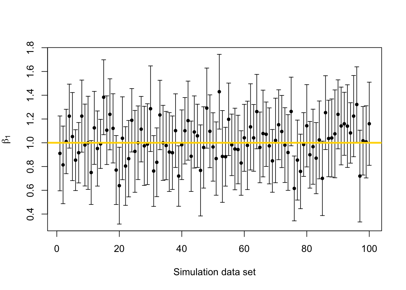
# Calculate the coverage probability
covered <- ifelse(sim.results[,2] < beta.truth[2] & sim.results[,3] > beta.truth[2],1,0)
mean(covered)
## [1] 0.94
12.5 Bootstrap confidence intervals
Google scholar demonstration
Motivation (see section 3.6 in Faraway (2014))
- Functions of parameters (i.e., “derived” quantities)
- Difficult to obtain the sampling distribution for non-linear functions of estimated parameters
- Further reading (Hesterberg 2015)
- Example: When do we expect the population to go extinct?
y <- c(63, 68, 61, 44, 103, 90, 107, 105, 76, 46, 60, 66, 58, 39, 64, 29, 37,
27, 38, 14, 38, 52, 84, 112, 112, 97, 131, 168, 70, 91, 52, 33, 33, 27,
18, 14, 5, 22, 31, 23, 14, 18, 23, 27, 44, 18, 19)
year <- 1965:2011
df <- data.frame(y = y, year = year)
plot(x = df$year, y = df$y, xlab = "Year", ylab = "Annual count", main = "",
col = "brown", pch = 20, xlim = c(1965, 2040))
m1 <- lm(y~year)
abline(m1)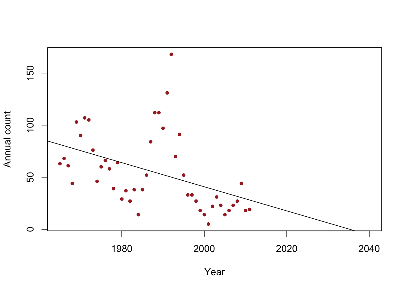
Non-parametric bootstrap (see Efron and Tibshirani (1994)).
- From a data set with n observations, take a sample of size n with replacement. For a linear model, the sample should include both the observed response (\(y_{i}\)) and covariates (\(x_{1}\),\(x_{2}\),…,\(x_{p}\)).
- Estimate the parameters for a statistical model using the sampled data from step 1.
- Save the estimates of interest. This could be parameters of interest (e.g., \(\boldsymbol{\beta}\)) or a a derived quantity (e.g., \(R^{2}\), \(\frac{1}{\boldsymbol{\beta}}\)).
- Repeats steps (1)-(3) \(m\) times.
Inference
- The \(m\) samples of the quantities of interest are samples from the empirical distribution.
- The empirical distribution can summarized using sample statistics (e.g., quantiles, mean, variance, etc). Conceptually, this is similar to Monte Carlo integration.
Example in R
library(latex2exp)
# Number of bootstrap samples (m)
m.boot <- 1000

# Create matrix to save empirical distribution of -beta2.hat/beta1.hat (expected time of extinction)
ed.extinct.hat <- matrix(,m.boot,1)

# Set random seed so results are the same if we run it again
# Results would be different due to random resampling of data
set.seed(1940)

# Start for loop for non-parametric boostrap
for(m in 1:m.boot){

  # Sample data with replacement
  # boot.sample gives the rows of df that we use for estimation
  boot.sample <- sample(1:nrow(df),replace=TRUE)

  # Make temporary data frame that contains the resamples
  df.temp <- df[boot.sample,]

  # Estimate parameters for df.temp
  m1 <- lm(y~year,data=df.temp)

  # Save estimate of -beta0.hat/beta1.hat (expected time of extinction)
  ed.extinct.hat[m,] <- -coef(m1)[1]/coef(m1)[2]
}
par(mar=c(5,4,7,2))
hist(ed.extinct.hat,col="grey",xlab="Year",main=TeX('Empirical distribuiton of $$-$$\\hat{\\frac{$\\beta_0}{$\\beta_1}}'),freq=FALSE,breaks=20)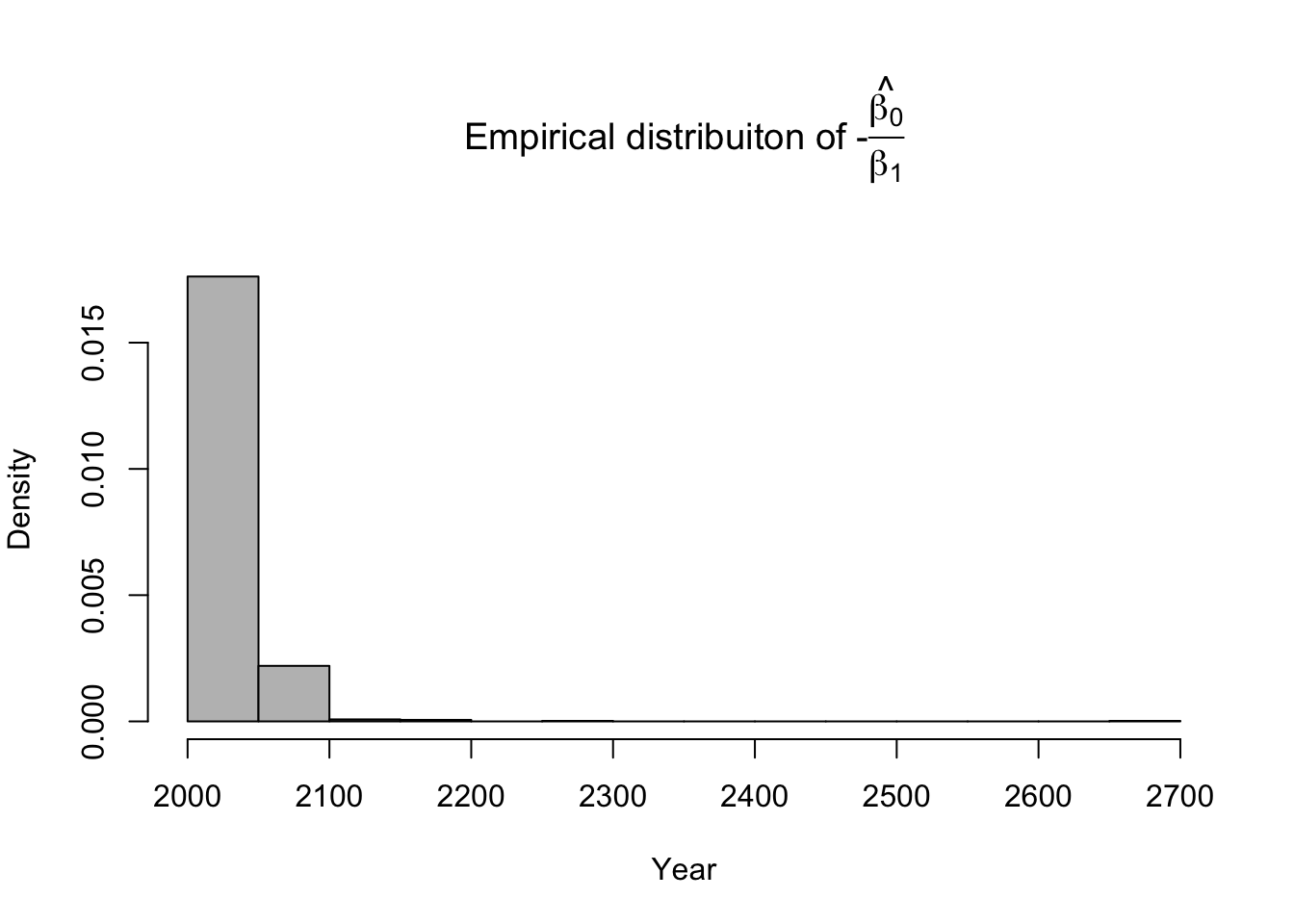
# 95% equal-tailed CI based on percentiles of the empirical distribution
quantile(ed.extinct.hat,prob=c(0.025,0.975))
## 2.5% 97.5% ## 2021.203 2077.168Example in R using the mosaic package
library(mosaic)

set.seed(1940)
bootstrap <- do(1000)*coef(lm(y~year,data=resample(df)))
head(bootstrap)
## Intercept year ## 1 1703.401 -0.8291862 ## 2 3017.102 -1.4887107 ## 3 2683.814 -1.3195092 ## 4 2595.994 -1.2778627 ## 5 2334.905 -1.1463994 ## 6 2011.819 -0.9811046# 95% equal-tailed CI based on percentiles of the empirical distribution quantile(-bootstrap[,1]/bootstrap[,2],prob=c(0.025,0.975))## 2.5% 97.5% ## 2021.203 2077.168confint(bootstrap,method="percentile") # Comparison of 95% CI with traditional approach## name lower upper level method estimate ## 1 year -1.623489 -0.6753815 0.95 percentile -1.15784confint(m1)[2,]## 2.5 % 97.5 % ## -1.9107236 -0.5405716
References
Efron, Bradley, and Robert J Tibshirani. 1994. An Introduction to the Bootstrap. CRC press.
Faraway, J. J. 2014. Linear Models with r. CRC Press.
Hesterberg, Tim C. 2015. “What Teachers Should Know about the Bootstrap: Resampling in the Undergraduate Statistics Curriculum.” The American Statistician 69 (4): 371–86.