14 Day 14 (June 22)
14.2 Confidence intervals for derived quantities
Demonstration of how not to do it.
y <- c(63, 68, 61, 44, 103, 90, 107, 105, 76, 46, 60, 66, 58, 39, 64, 29, 37,
27, 38, 14, 38, 52, 84, 112, 112, 97, 131, 168, 70, 91, 52, 33, 33, 27,
18, 14, 5, 22, 31, 23, 14, 18, 23, 27, 44, 18, 19)
year <- 1965:2011
df <- data.frame(y = y, year = year)
plot(x = df$year, y = df$y, xlab = "Year", ylab = "Annual count", main = "",
col = "brown", pch = 20, xlim = c(1965, 2040))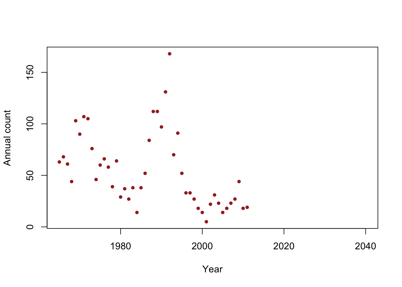
m1 <- lm(y~year,data=df)
coef(m1)
## (Intercept) year ## 2356.48797 -1.15784confint(m1,level=0.95)## 2.5 % 97.5 % ## (Intercept) 929.80699 3783.1689540 ## year -1.87547 -0.4402103# This is ok! beta0.hat <- as.numeric(coef(m1)[1]) beta1.hat <- as.numeric(coef(m1)[2]) extinct.date.hat <- -beta0.hat/beta1.hat extinct.date.hat## [1] 2035.245# This is not ok! beta0.hat.li <- confint(m1)[1,1] beta1.hat.li <- confint(m1)[2,1] extinct.date.li <- -beta0.hat.li/beta1.hat.li extinct.date.li## [1] 495.7729beta0.hat.ui <- confint(m1)[1,2] beta1.hat.ui <- confint(m1)[2,2] extinct.date.ui <- -beta0.hat.ui/beta1.hat.ui extinct.date.ui## [1] 8594.004The delta method
- See (Ver Hoef 2012) and (Powell 2007) for more info
library(msm)

y <- c(63, 68, 61, 44, 103, 90, 107, 105, 76, 46, 60, 66, 58, 39, 64, 29, 37,
   27, 38, 14, 38, 52, 84, 112, 112, 97, 131, 168, 70, 91, 52, 33, 33, 27,
   18, 14, 5, 22, 31, 23, 14, 18, 23, 27, 44, 18, 19)
year <- 1965:2011
df <- data.frame(y = y, year = year)
plot(x = df$year, y = df$y, xlab = "Year", ylab = "Annual count", main = "",
 col = "brown", pch = 20, xlim = c(1965, 2040))
m1 <- lm(y~year,data=df)
coef(m1)
## (Intercept) year ## 2356.48797 -1.15784confint(m1,level=0.95)## 2.5 % 97.5 % ## (Intercept) 929.80699 3783.1689540 ## year -1.87547 -0.4402103beta0.hat <- as.numeric(coef(m1)[1]) beta1.hat <- as.numeric(coef(m1)[2]) extinct.date.hat <- -beta0.hat/beta1.hat extinct.date.hat## [1] 2035.245extinct.date.se <- deltamethod(~-x1/x2, mean=coef(m1), cov=vcov(m1)) extinct.date.ci <- c(extinct.date.hat-1.96*extinct.date.se, extinct.date.hat+1.96*extinct.date.se) extinct.date.ci## [1] 2005.598 2064.892Live example
References
Powell, Larkin A. 2007. “Approximating Variance of Demographic Parameters Using the Delta Method: A Reference for Avian Biologists.” The Condor 109 (4): 949–54.
Ver Hoef, Jay M. 2012. “Who Invented the Delta Method?” The American Statistician 66 (2): 124–27.