19 Day 19 (June 29)

19.1 Announcements

• Read Chs. 14, 15 and 16 in linear models with R

19.2 Regression and ANOVA

• Review of the linear model
• Regression, ANOVA, and t-test as special cases of the linear model
  • Write the regression and ANOVA model out on white board

19.3 T-test

• Common statistical test taught in introductory statistics classes

  • Linear model representation

  • Example: comparing two means

    library(faraway)
    df.plant <- PlantGrowth[-c(1:10),]
    df.plant$group <- factor(df.plant$group) 
    
    boxplot(weight ~ group,df.plant,col="grey",ylim=c(0,7))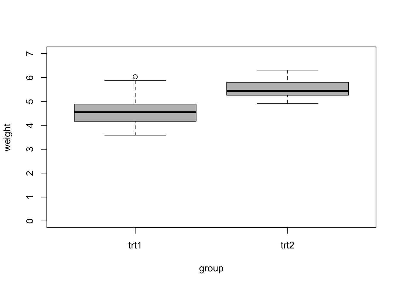

    

    aggregate(weight ~ group, FUN=mean,data=df.plant)

    ##   group weight
    ## 1  trt1  4.661
    ## 2  trt2  5.526

  • Use t.test() function in R.

    t.test(weight ~ group-1,data = df.plant,var.equal = TRUE)

    ## 
    ##  Two Sample t-test
    ## 
    ## data:  weight by group
    ## t = -3.0101, df = 18, p-value = 0.007518
    ## alternative hypothesis: true difference in means between group trt1 and group trt2 is not equal to 0
    ## 95 percent confidence interval:
    ##  -1.4687336 -0.2612664
    ## sample estimates:
    ## mean in group trt1 mean in group trt2 
    ##              4.661              5.526

  • Use lm() function in R.

    # With "intercept"
    m1 <- lm(weight ~ group,data = df.plant)
    summary(m1)

    ## 
    ## Call:
    ## lm(formula = weight ~ group, data = df.plant)
    ## 
    ## Residuals:
    ##     Min      1Q  Median      3Q     Max 
    ## -1.0710 -0.3573 -0.0910  0.2402  1.3690 
    ## 
    ## Coefficients:
    ##             Estimate Std. Error t value Pr(>|t|)    
    ## (Intercept)   4.6610     0.2032   22.94 8.93e-15 ***
    ## grouptrt2     0.8650     0.2874    3.01  0.00752 ** 
    ## ---
    ## Signif. codes:  0 '***' 0.001 '**' 0.01 '*' 0.05 '.' 0.1 ' ' 1
    ## 
    ## Residual standard error: 0.6426 on 18 degrees of freedom
    ## Multiple R-squared:  0.3348, Adjusted R-squared:  0.2979 
    ## F-statistic: 9.061 on 1 and 18 DF,  p-value: 0.007518

    # Without "intercept"
    m2 <- lm(weight ~ group-1,data = df.plant)
    summary(m2)

    ## 
    ## Call:
    ## lm(formula = weight ~ group - 1, data = df.plant)
    ## 
    ## Residuals:
    ##     Min      1Q  Median      3Q     Max 
    ## -1.0710 -0.3573 -0.0910  0.2402  1.3690 
    ## 
    ## Coefficients:
    ##           Estimate Std. Error t value Pr(>|t|)    
    ## grouptrt1   4.6610     0.2032   22.94 8.93e-15 ***
    ## grouptrt2   5.5260     0.2032   27.20 4.52e-16 ***
    ## ---
    ## Signif. codes:  0 '***' 0.001 '**' 0.01 '*' 0.05 '.' 0.1 ' ' 1
    ## 
    ## Residual standard error: 0.6426 on 18 degrees of freedom
    ## Multiple R-squared:  0.986,  Adjusted R-squared:  0.9844 
    ## F-statistic: 632.9 on 2 and 18 DF,  p-value: < 2.2e-16