36 Day 36 (July 26)
36.2 The Bayesian Linear Model
The model
- Distribution of the data: “\(\mathbf{y}\) given \(\boldsymbol{\beta}\) and \(\sigma_{\varepsilon}^{2}\)” \[\mathbf{y}|\boldsymbol{\beta},\sigma_{\varepsilon}^{2}\sim\text{N}(\mathbf{X}\boldsymbol{\beta},\sigma_{\varepsilon}^{2}\mathbf{I})\] This is also sometimes called the data model.
- Distribution of the parameters: \(\boldsymbol{\beta}\) and \(\sigma_{\varepsilon}^{2}\) \[\boldsymbol{\beta}\sim\text{N}(\mathbf{0},\sigma_{\beta}^{2}\mathbf{I})\] \[\sigma_{\varepsilon}^{2}\sim\text{inverse gamma}(q,r)\]
Computations and statistical inference
- Using Bayes rule (Bayes 1763) we can obtain the joint posterior distribution
\[[\boldsymbol{\beta},\sigma_{\varepsilon}^{2}|\mathbf{y}]=\frac{[\mathbf{y}|\boldsymbol{\beta},\sigma_{\varepsilon}^{2}][\boldsymbol{\beta}][\sigma_{\varepsilon}^{2}]}{\int\int [\mathbf{y}|\boldsymbol{\beta},\sigma_{\varepsilon}^{2}][\boldsymbol{\beta}][\sigma_{\varepsilon}^{2}]d\boldsymbol{\beta}d\sigma_{\varepsilon}^{2}}\]
- Statistical inference about a paramters is obtained from the marginal posterior distributions \[[\boldsymbol{\beta}|\mathbf{y}]=\int[\boldsymbol{\beta},\sigma_{\varepsilon}^{2}|\mathbf{y}]d\sigma_{\varepsilon}^{2}\] \[[\sigma_{\varepsilon}^{2}|\mathbf{y}]=\int[\boldsymbol{\beta},\sigma_{\varepsilon}^{2}|\mathbf{y}]d\boldsymbol{\beta}\]
- In practice it is difficult to find closed-form solutions for the marginal posterior distributions, but easy to find closed-form solutions for the conditional posterior distribtuions.
- Full-conditional distribtuions: \(\boldsymbol{\beta}\) and \(\sigma_{\varepsilon}^{2}\) \[\boldsymbol{\beta}|\sigma_{\varepsilon}^{2},\mathbf{y}\sim\text{N}\bigg{(}\big{(}\mathbf{X}^{\prime}\mathbf{X}+\frac{1}{\sigma_{\beta}^{2}}\mathbf{I}\big{)}^{-1}\mathbf{X}^{\prime}\mathbf{y},\sigma_{\varepsilon}^{2}\big{(}\mathbf{X}^{\prime}\mathbf{X}+\frac{1}{\sigma_{\beta}^{2}}\mathbf{I}\big{)}^{-1}\bigg{)}\] \[\sigma_{\varepsilon}^{2}|\mathbf{\boldsymbol{\beta}},\mathbf{y}\sim\text{inverse gamma}\left(q+\frac{n}{2},(r+\frac{1}{2}(\mathbf{y}-\mathbf{X}\boldsymbol{\beta})^{'}(\mathbf{y}-\mathbf{X}\boldsymbol{\beta}))^-1\right)\]
- Gibbs sampler for the Bayesian linear model
- Write out on the whiteboard
- Using Bayes rule (Bayes 1763) we can obtain the joint posterior distribution
\[[\boldsymbol{\beta},\sigma_{\varepsilon}^{2}|\mathbf{y}]=\frac{[\mathbf{y}|\boldsymbol{\beta},\sigma_{\varepsilon}^{2}][\boldsymbol{\beta}][\sigma_{\varepsilon}^{2}]}{\int\int [\mathbf{y}|\boldsymbol{\beta},\sigma_{\varepsilon}^{2}][\boldsymbol{\beta}][\sigma_{\varepsilon}^{2}]d\boldsymbol{\beta}d\sigma_{\varepsilon}^{2}}\]
Example: Mauna Loa Observatory carbon dioxide data
url <- "ftp://aftp.cmdl.noaa.gov/products/trends/co2/co2_annmean_mlo.txt"
df <- read.table(url,header=FALSE)
colnames(df) <- c("year","meanCO2","unc")
plot(x = df$year, y = df$meanCO2, xlab = "Year", ylab = expression("Mean annual "*CO[2]*" concentration"),col="black",pch=20)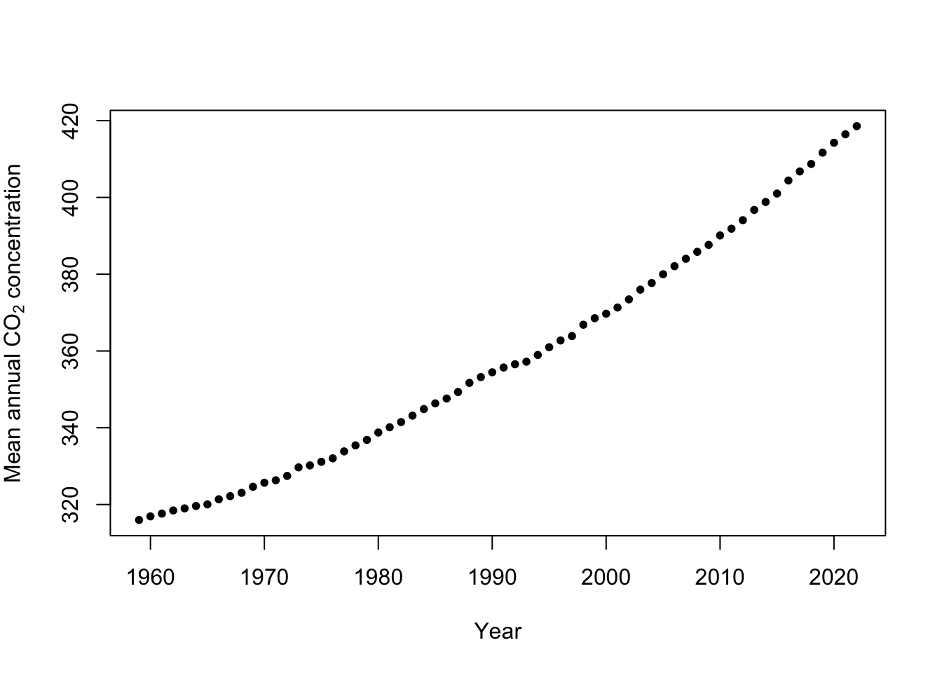
- Gibb sampler
# Preliminary steps
library(mvnfast) # Required package to sample from multivariate normal distribution
## ## Attaching package: 'mvnfast'## The following objects are masked from 'package:mgcv': ## ## dmvn, rmvny <- df$meanCO2 # Response variable X <- model.matrix(~year, data=df) # Design matrix n <- length(y) # Number of observations p <- 2 # Dimensions of beta m.draws <- 5000 #Number of MCMC samples to draw samples <- as.data.frame(matrix(,m.draws,3)) # Samples of the parameters we will save colnames(samples) <- c(colnames(X),"sigma2") sigma2.e <- 1 # Starting values for sigma2 sigma2.beta <- 10^9 #Prior variance for beta q <- 2.01 #Inverse gamma prior with E() = 1/(r*(q-1)) and Var()= 1/(r^2*(q-1)^2*(q-2)) r <- 1 # MCMC algorithm for(m in 1:m.draws){ # Sample beta from full-conditional distribution H <- solve(t(X)%*%X + diag(1/sigma2.beta,p)) h <- t(X)%*%y beta <- t(rmvn(1,H%*%h,sigma2.e*H)) # Sample sigma from full-conditional distribution q.temp <- q+n/2 r.temp <- (1/r+t(y-X%*%beta)%*%(y-X%*%beta)/2)^-1 sigma2.e <- 1/rgamma(1,q.temp,,r.temp) # Save samples of beta and sigma samples[m,] <- c(beta,sigma2.e) } # Look a histograms of posterior distributions par(mfrow=c(3,1),mar=c(5,6,1,1)) hist(samples[,1],xlab=expression(beta[0]*"|"*bold(y)),ylab=expression("["*beta[0]*"|"*bold(y)*"]"),freq=FALSE,col="grey",main="",breaks=30) hist(samples[,2],xlab=expression(beta[1]*"|"*bold(y)),ylab=expression("["*beta[1]*"|"*bold(y)*"]"),freq=FALSE,col="grey",main="",breaks=30) hist(samples[,3],xlab=expression(sigma^2*"|"*bold(y)),ylab=expression("["*sigma^2*"|"*bold(y)*"]"),freq=FALSE,col="grey",main="",breaks=30)
# Mean of the posterior distribution
colMeans(samples[,1:2])
## (Intercept) year ## -2882.979210 1.628374# Compare to results obtained from lm function m1 <- lm(y~X-1) coef(m1)## X(Intercept) Xyear ## -2881.953419 1.627857- Using the R package MCMCpack
library(MCMCpack)
samples <- MCMCregress(y ~ X - 1,
                         burnin = 0,mcmc = 5000 ,
                         b0 = 0,B0 = 1/sigma2.beta,
                         c0 = q, d0 = 1/r)
samples <- samples[1:5000,] # Extract samples from the posterior for beta and sigma2 from MCMCregress output

# Look a histograms of posterior distributions
par(mfrow=c(3,1),mar=c(5,6,1,1))
hist(samples[,1],xlab=expression(beta[0]*"|"*bold(y)),ylab=expression("["*beta[0]*"|"*bold(y)*"]"),freq=FALSE,col="grey",main="",breaks=30)
hist(samples[,2],xlab=expression(beta[1]*"|"*bold(y)),ylab=expression("["*beta[1]*"|"*bold(y)*"]"),freq=FALSE,col="grey",main="",breaks=30)
hist(samples[,3],xlab=expression(sigma^2*"|"*bold(y)),ylab=expression("["*sigma^2*"|"*bold(y)*"]"),freq=FALSE,col="grey",main="",breaks=30)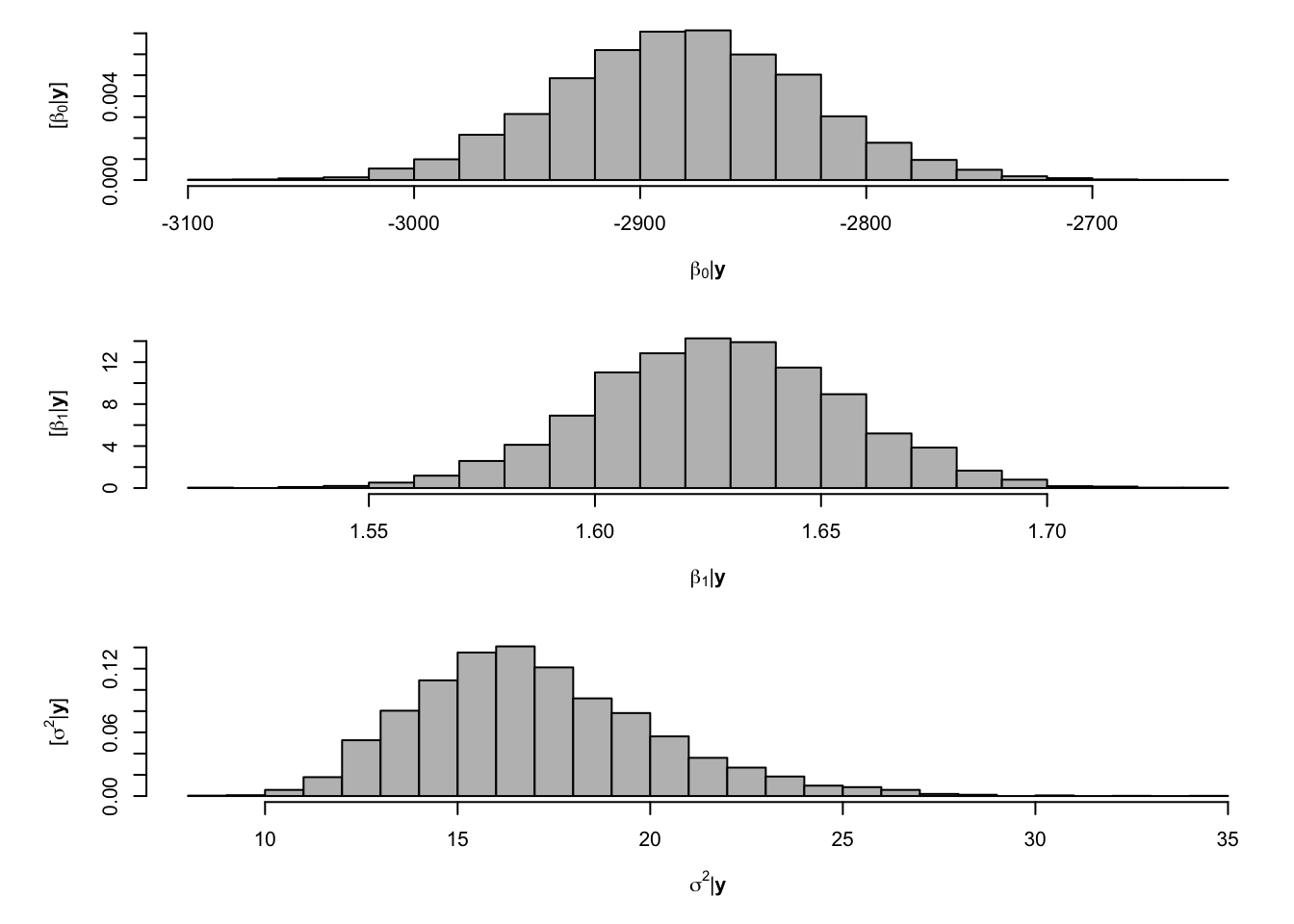
# Mean of the posterior distribution
colMeans(samples[,1:2])
## X(Intercept) Xyear ## -2881.026502 1.627389