41 Assignment 2 (Guide)
A mathematical model is a simplification and description of some real-world phenomenon. The model is usually expressed and communicated using a mathematical equation. The equation is deterministic and does not allow for the real-world phenomenon to have any randomness in it.
A statistical model is a simplification and description of some real-world phenomenon. The model is usually expressed and communicated using a mathematical equation and a probability density/mass function (e.g., the normal distribution). The combination of the mathematical equation and probability density/mass function enables to model to be stochastic and account for randomness in a real-world phenomenon that the model describes.
Everyone did great answering this question!!!
A <- matrix(c(1,2,3,2,5,6,3,6,9),3,3,byrow=TRUE) B <- diag(1,3) C <- t(A)A+C## [,1] [,2] [,3] ## [1,] 2 4 6 ## [2,] 4 10 12 ## [3,] 6 12 18A-C## [,1] [,2] [,3] ## [1,] 0 0 0 ## [2,] 0 0 0 ## [3,] 0 0 0A%*%B## [,1] [,2] [,3] ## [1,] 1 2 3 ## [2,] 2 5 6 ## [3,] 3 6 9solve(A+B)%*%(C+B)## [,1] [,2] [,3] ## [1,] 1 6.661338e-16 4.440892e-16 ## [2,] 0 1.000000e+00 0.000000e+00 ## [3,] 0 0.000000e+00 1.000000e+00Which of the models below are a linear statistical model? Please justify your answer using words.
- Multiple answers are correct here. This is a linear model because the only non-linear part is where the predictor variable (i.e., \(\mathbf{x}\)) is squared. Any linear or non-linear transformation of the predictor variable does not change if a model is linear or non-linear. Another correct answer is that this is not a linear model because the error term (i.e., \(\boldsymbol{\varepsilon}\)) is missing. If the error term was not missing, then it would be a linear model.
- This is a linear model because the only non-linear part is where Euler’s number (i.e., \(e\)) is raised to the \(\mathbf{x}\) power. Any linear or non-linear transformation of the predictor variable does not change if a model is linear or non-linear.
- This is not a linear model because Euler’s number is raised to the parameter \(\beta_{1}\) power (i.e., the parameter shows up in the model inside of a non-linear function).
- Multiple answers are correct here. This is not a linear model because the parameter shows up in the model inside of a non-linear function. Another correct answer is that you can easily simplify the model and show that it is the same as \(\mathbf{y}=\beta_{0}+\beta_{1}\mathbf{x}+\boldsymbol{\varepsilon}.\)
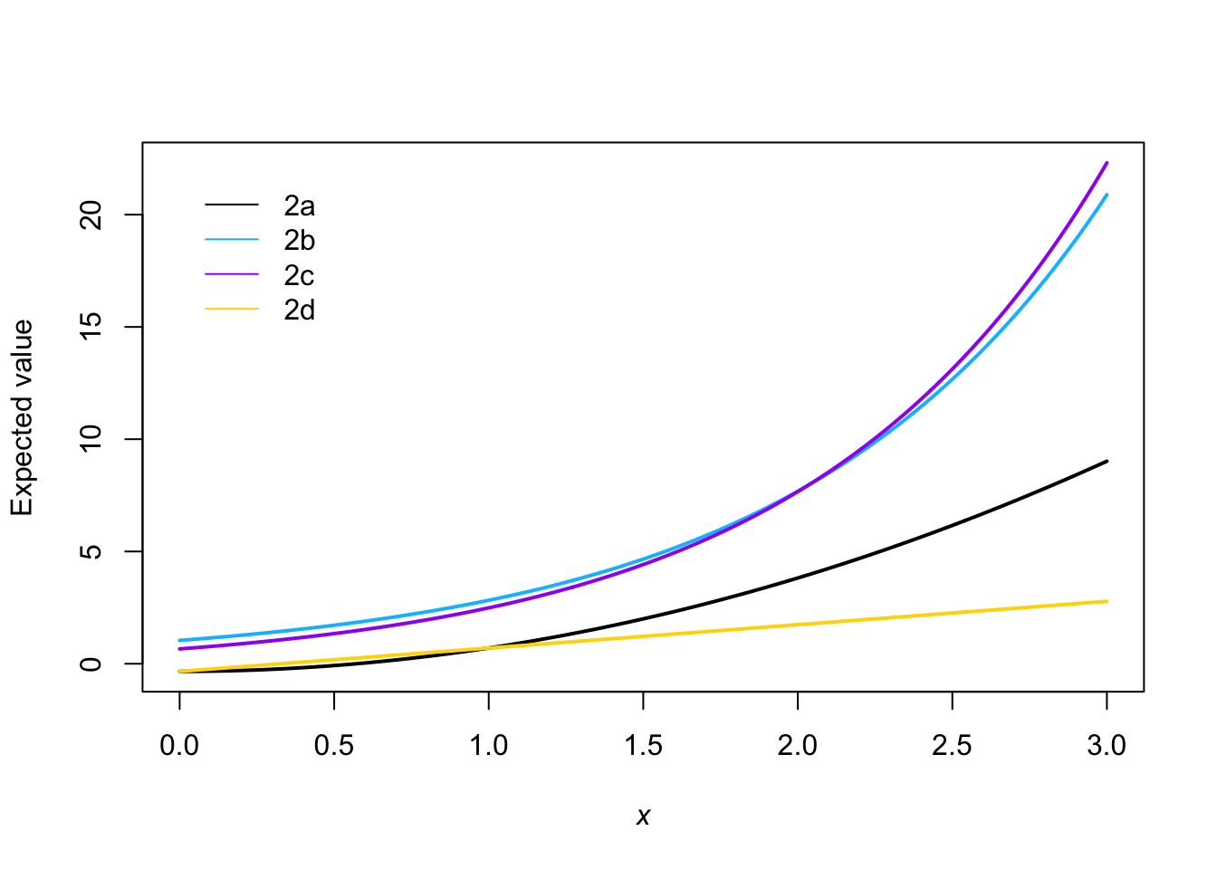
x <- seq(0,3,by=0.01)
beta <- c(-0.34,1.04)
E.y_a <- beta[1]+beta[2]*x^2
E.y_b <- beta[2]*exp(x)
E.y_c <- beta[1]+exp(beta[2]*x)
E.y_d <- beta[1]+beta[2]*x
col <- c("black","deepskyblue","purple","gold")

plot(x,E.y_a,ylim=c(range(E.y_a,E.y_b,E.y_c,E.y_d)),
 typ="l",col=col[1],
 xlab=expression(italic(x)),
 ylab="Expected value",lwd=2)
points(x,E.y_b,typ="l",col=col[2],lwd=2)
points(x,E.y_c,typ="l",col=col[3],lwd=2)
points(x,E.y_d,typ="l",col=col[4],lwd=2)
legend(x=0,y=22,legend=c("2a","2b","2c","2d"),bty="n",lty=1,
   col=col)