29 Day 29 (July 17)
29.2 Collinearity
When two or more of the predictor variables (i.e., columns of \(\mathbf{X}\)) are correlated, the predictors are said to be collinear. Also called
- Collinearity
- Multicollinearity
- Correlation among predictors/covariates
- Partial parameter identifiability
Collinearity cause coefficient estimates (i.e., \(\hat{\boldsymbol{\beta}}\) to change when a collinear predictor is removed (or added) to the model.
- Extremely common problem with observational data and data collected from poorly designed experiments.
Example
- The data
library(httr)
library(readxl)

url <- "https://doi.org/10.1371/journal.pone.0148743.s005"
GET(url, write_disk(path <- tempfile(fileext = ".xls")))
df1 <- read_excel(path=path,sheet = "Data", col_names=TRUE,col_types="numeric") notes <- read_excel(path=path,sheet = "Notes", col_names=FALSE)head(df1)## # A tibble: 6 × 9 ## States Year CDEP WKIL WPOP BRPA NCAT SDEP NSHP ## <dbl> <dbl> <dbl> <dbl> <dbl> <dbl> <dbl> <dbl> <dbl> ## 1 1 1987 6 4 10 2 9736 10 1478 ## 2 1 1988 0 0 14 1 9324 0 1554 ## 3 1 1989 3 1 12 1 9190 0 1572 ## 4 1 1990 5 1 33 3 8345 0 1666 ## 5 1 1991 2 0 29 2 8733 2 1639 ## 6 1 1992 1 0 41 4 9428 0 1608notes## # A tibble: 9 × 2 ## ...1 ...2 ## <chr> <chr> ## 1 Year <NA> ## 2 State 1=Montana,2=Wyoming,3=Idaho ## 3 Cattle depredated CDEP ## 4 Sheep depredated SDEP ## 5 Wolf population WPOP ## 6 Wolves killed WKIL ## 7 Breeding pairs BRPA ## 8 Number of cattleA* NCAT ## 9 Number of SheepB* NSHPFit a linear model
m1 <- lm(CDEP ~ NCAT + WPOP,data=df1)
summary(m1)
## ## Call: ## lm(formula = CDEP ~ NCAT + WPOP, data = df1) ## ## Residuals: ## Min 1Q Median 3Q Max ## -40.289 -8.147 -3.475 2.678 92.257 ## ## Coefficients: ## Estimate Std. Error t value Pr(>|t|) ## (Intercept) -3.8455597 8.1697216 -0.471 0.64 ## NCAT 0.0009372 0.0010363 0.904 0.37 ## WPOP 0.1031119 0.0119644 8.618 7.51e-12 *** ## --- ## Signif. codes: 0 '***' 0.001 '**' 0.01 '*' 0.05 '.' 0.1 ' ' 1 ## ## Residual standard error: 20.23 on 56 degrees of freedom ## (3 observations deleted due to missingness) ## Multiple R-squared: 0.5855, Adjusted R-squared: 0.5707 ## F-statistic: 39.55 on 2 and 56 DF, p-value: 1.951e-11- Killing wolves should reduce the number of cattle depredated, right? Let’s add the number of wolves killed to our model.
m2 <- lm(CDEP ~ NCAT + WPOP + WKIL,data=df1)
summary(m2)
## ## Call: ## lm(formula = CDEP ~ NCAT + WPOP + WKIL, data = df1) ## ## Residuals: ## Min 1Q Median 3Q Max ## -18.519 -8.549 -1.588 4.049 79.041 ## ## Coefficients: ## Estimate Std. Error t value Pr(>|t|) ## (Intercept) 13.901373 6.511267 2.135 0.0372 * ## NCAT -0.001385 0.000830 -1.669 0.1008 ## WPOP 0.011868 0.015724 0.755 0.4536 ## WKIL 0.683946 0.097769 6.996 3.84e-09 *** ## --- ## Signif. codes: 0 '***' 0.001 '**' 0.01 '*' 0.05 '.' 0.1 ' ' 1 ## ## Residual standard error: 14.85 on 55 degrees of freedom ## (3 observations deleted due to missingness) ## Multiple R-squared: 0.7807, Adjusted R-squared: 0.7687 ## F-statistic: 65.25 on 3 and 55 DF, p-value: < 2.2e-16- What happened?!
cor(df1[,c(4,5,7)],use="complete.obs")## WKIL WPOP NCAT ## WKIL 1.00000000 0.7933354 -0.04460099 ## WPOP 0.79333543 1.0000000 -0.34440797 ## NCAT -0.04460099 -0.3444080 1.00000000Some analytical results
- Assume the linear model \[\mathbf{y}=\beta_{1}\mathbf{x}+\beta_{2}\mathbf{z}+\boldsymbol{\varepsilon}\] where \(\boldsymbol{\varepsilon}\sim\text{N}(\mathbf{0},\sigma^{2}\mathbf{I})\)
- Assume that the predictors \(\mathbf{x}\) and \(\mathbf{z}\) are correlated (i.e., are not orthogonal \(\mathbf{x}^{\prime}\mathbf{z}\neq 0\) and \(\mathbf{z}^{\prime}\mathbf{x}\neq 0\)).
- Then \[\hat{\beta}_1 = (\mathbf{x}^{\prime}\mathbf{x}\times\mathbf{z}^{\prime}\mathbf{z} - \mathbf{x}^{\prime}\mathbf{z}\times\mathbf{z}^{\prime}\mathbf{x})^{-1}((\mathbf{z}^{\prime}\mathbf{z})\mathbf{x}^{\prime} - (\mathbf{x}^{\prime}\mathbf{z})\mathbf{z}^{\prime})\mathbf{y}\] and \[\hat{\beta}_2 = (\mathbf{z}^{\prime}\mathbf{z}\times\mathbf{x}^{\prime}\mathbf{x} - \mathbf{z}^{\prime}\mathbf{x}\times\mathbf{x}^{\prime}\mathbf{z})^{-1}((\mathbf{x}^{\prime}\mathbf{x})\mathbf{z}^{\prime} - (\mathbf{z}^{\prime}\mathbf{x})\mathbf{x}^{\prime})\mathbf{y}.\] The variance is \[\text{Var}(\hat{\beta}_{1})=\sigma^{2}\bigg{(}\frac{1}{1-R^{2}_{xz}}\bigg{)}\frac{1}{\sum_{i=1}^{n}(x_{i}-\bar{x})^{2}}\] \[\text{Var}(\hat{\beta}_{2})=\sigma^{2}\bigg{(}\frac{1}{1-R^{2}_{xz}}\bigg{)}\frac{1}{\sum_{i=1}^{n}(z_{i}-\bar{z})^{2}}\]where \(R^{2}_{xz}\) is the correlation between \(\mathbf{x}\) and \(\mathbf{z}\) (see pg. 107 in Faraway (2014)).
Take away message
- \(\hat{\beta}_i\) is the unbiased and minimum variance estimator assuming all predictors for \(\beta_i \neq 0\) are in the model.
- \(\hat{\beta}_i\) depends on the other predictors in the model.
- Correlation among predictors increases the variance of \(\hat{\beta}_i\).
- Known as the variance inflation factor
- Collinearity is ubiquitous in any model with correlated predictors
library(faraway)
vif(m2)
## NCAT WPOP WKIL ## 1.350723 3.637257 3.212207
29.3 Model selection
Recall that all inference is conditional on the statistical model that we have chosen to use.
- Components of a statistical model
- Are the assumptions met?
- Are there better models we could have used?
- What should you do if you have two or more competing models?
Information criterion
- Motivation: Adjusted \(R^2\)
- Recall \[\hat{R}^{2}=1-\frac{(\mathbf{y}-\mathbf{X}\hat{\boldsymbol{\beta}})^{\prime}(\mathbf{y}-\mathbf{X}\hat{\boldsymbol{\beta})}}{(\mathbf{y}-\mathbf{1}\hat{\beta}_{0})^{\prime}(\mathbf{y}-\mathbf{1}\hat{\beta}_{0})}\]
- As we add more predictors to \(\mathbf{X}\), \(R^{2}\) monotonically increases when calculated using in-sample data.
- Calculating \(R^{2}\) using in-sample data results in a biased estimator of the \(R^{2}\) calculated using “out-of-sample” (i.e., \(\text{E}(\hat{R}_{\text{in-sample}}^{2})\neq R_{\text{out-of-sample}}^{2}\))
- Adjusted \(R^{2}\) is a biased corrected version of \(R^{2}\). \[\hat{R}^{2}_{\text{adjusted}}=1-\bigg{(}\frac{n-1}{n-p}\bigg{)}\frac{(\mathbf{y}-\mathbf{X}\hat{\boldsymbol{\beta}})^{\prime}(\mathbf{y}-\mathbf{X}\hat{\boldsymbol{\beta})}}{(\mathbf{y}-\mathbf{1}\hat{\beta}_{0})^{\prime}(\mathbf{y}-\mathbf{1}\hat{\beta}_{0})}\]
- Many different estimators exist for adjusted \(R^{2}\)
- Different assumptions lead to different estimators
- Gelman, Hwang, and Vehtari (2014) on estimating out-of-sample predictive accuracy using in-sample data
- “We know of no approximation that works in general….Each of these methods has flaws, which tells us that any predictive accuracy measure that we compute will be only approximate”
- “One difficulty is that all the proposed measures are attempting to perform what is, in general, an impossible task: to obtain an unbiased (or approximately unbiased) and accurate measure of out-of-sample prediction error that will be valid over a general class of models…”
- Motivation: Adjusted \(R^2\)
Akaike’s Information Criterion
- The log-likelihood as a scoring rule \[\mathcal{l}(\boldsymbol{\theta}|\mathbf{y})\]
- The log-likelihood for the linear model \[\mathcal{l}(\boldsymbol{\beta},\sigma^2|\mathbf{y})=-\frac{n}{2}\text{ log}(2\pi\sigma^2) - \frac{1}{2\sigma^2}\sum_{i=1}^{n}(y_{i} - \mathbf{x}_{i}^{\prime}\boldsymbol{\beta})^2.\]
- Like \(R^2\), \(\mathcal{l}(\boldsymbol{\beta},\sigma^2|\mathbf{y})\) can be used to measure predictive accuracy on in-sample or out of sample data.
- Unlike \(R^2\), the log-likelihood is a general scoring rule. For example, let \(\mathbf{y} \sim \text{Bernoulli}(p)\) then \[\sum_{i=1}^{n}y_{i}\text{log}(p)+(1-y_{i})\text{log}({1-p}).\]
- The log-likelihood is a relative score and can be difficult to interpret.
- AIC uses the in-sample log-likelihood, but achieves an (asymptotically) unbiased estimate the log-likelihood on the out-of-sample data by adding a bias correction. The statistic is then multiplied by negative two \[AIC=-2\mathcal{l}(\boldsymbol{\theta}|\mathbf{y}) + 2q\]
- What is a meaninful difference in AIC?
- AIC is a derived quanitity. Just like \(R^2\) we can and should get measures of uncertainty (e.g., 95% CI).
Example
- Motivation: Annual mean temperature in Ann Arbor Michigan
library(faraway)
plot(aatemp$year,aatemp$temp,xlab="Year",ylab="Annual mean temperature",pch=20,col=rgb(0.5,0.5,0.5,0.7))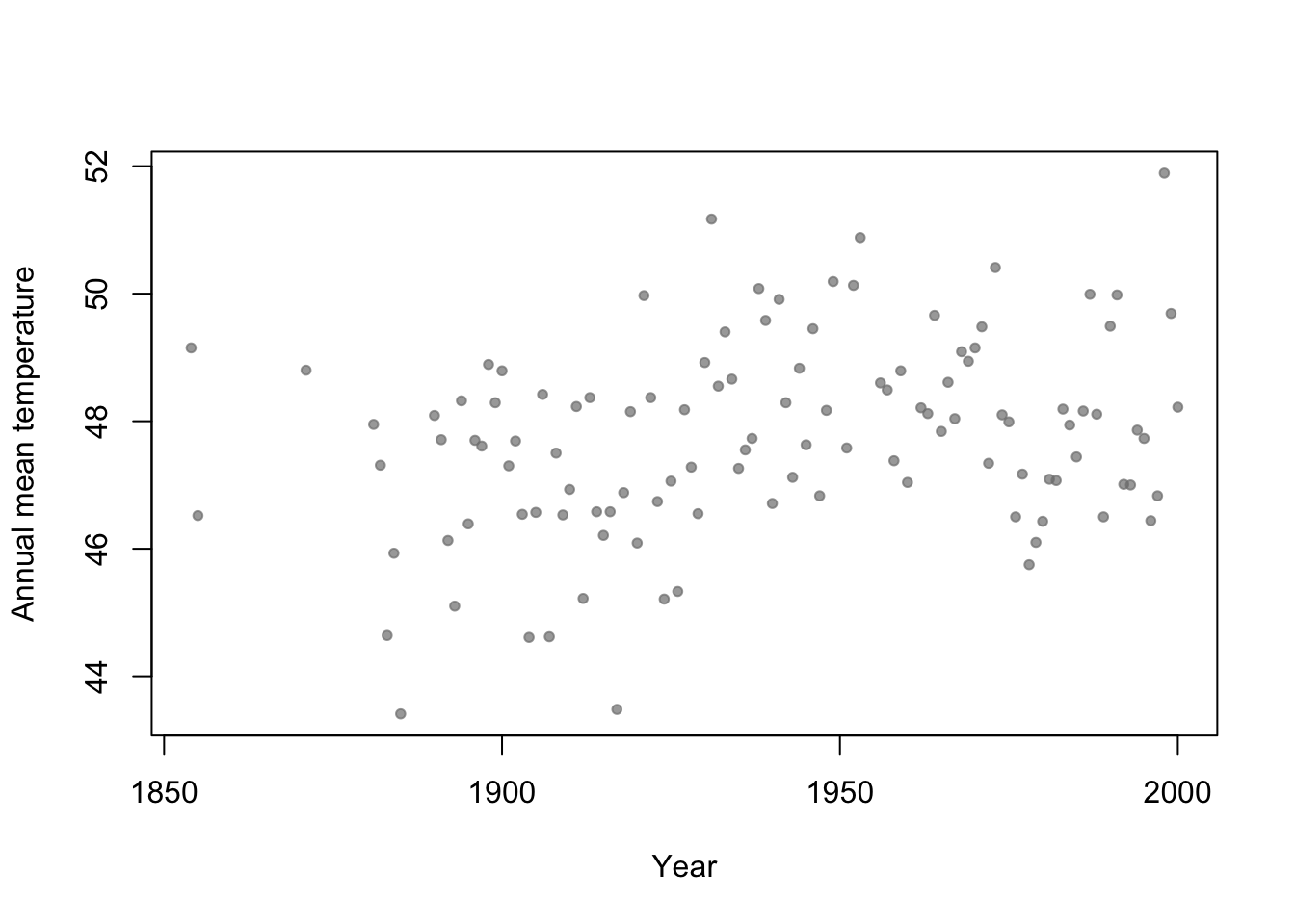
df.in_sample <- aatemp # Use all years for in-sample data

# Intercept only model
m1 <- lm(temp ~ 1,data=df.in_sample)

# Simple regression model
m2 <- lm(temp ~ year,data=df.in_sample)

par(mfrow=c(1,1))
# Plot predictions (in-sample)
plot(df.in_sample$year,df.in_sample$temp,main="In-sample",xlab="Year",ylab="Annual mean temperature",ylim=c(44,52),pch=20,col=rgb(0.5,0.5,0.5,0.7))
lines(df.in_sample$year,predict(m2))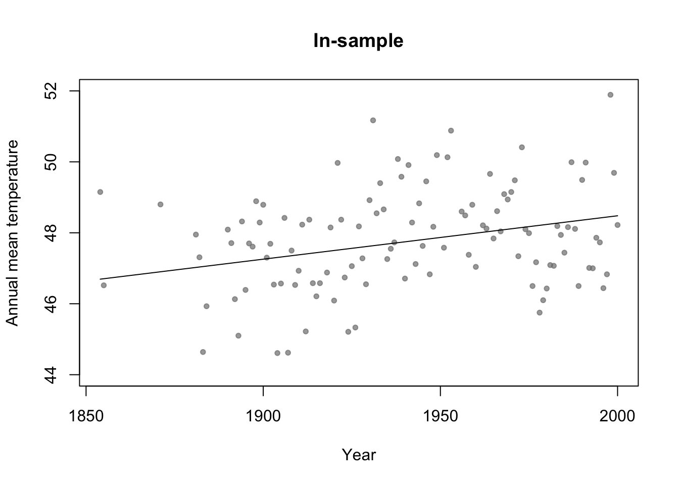
# Broken stick basis function
f1 <- function(x,c){ifelse(x<c,c-x,0)}
f2 <- function(x,c){ifelse(x>=c,x-c,0)}
m3 <- lm(temp ~ f1(year,1930) + f2(year,1930),data=df.in_sample)

par(mfrow=c(1,1))
# Plot predictions (in-sample)
plot(df.in_sample$year,df.in_sample$temp,main="In-sample",xlab="Year",ylab="Annual mean temperature",ylim=c(44,52),pch=20,col=rgb(0.5,0.5,0.5,0.7))
lines(df.in_sample$year,predict(m3))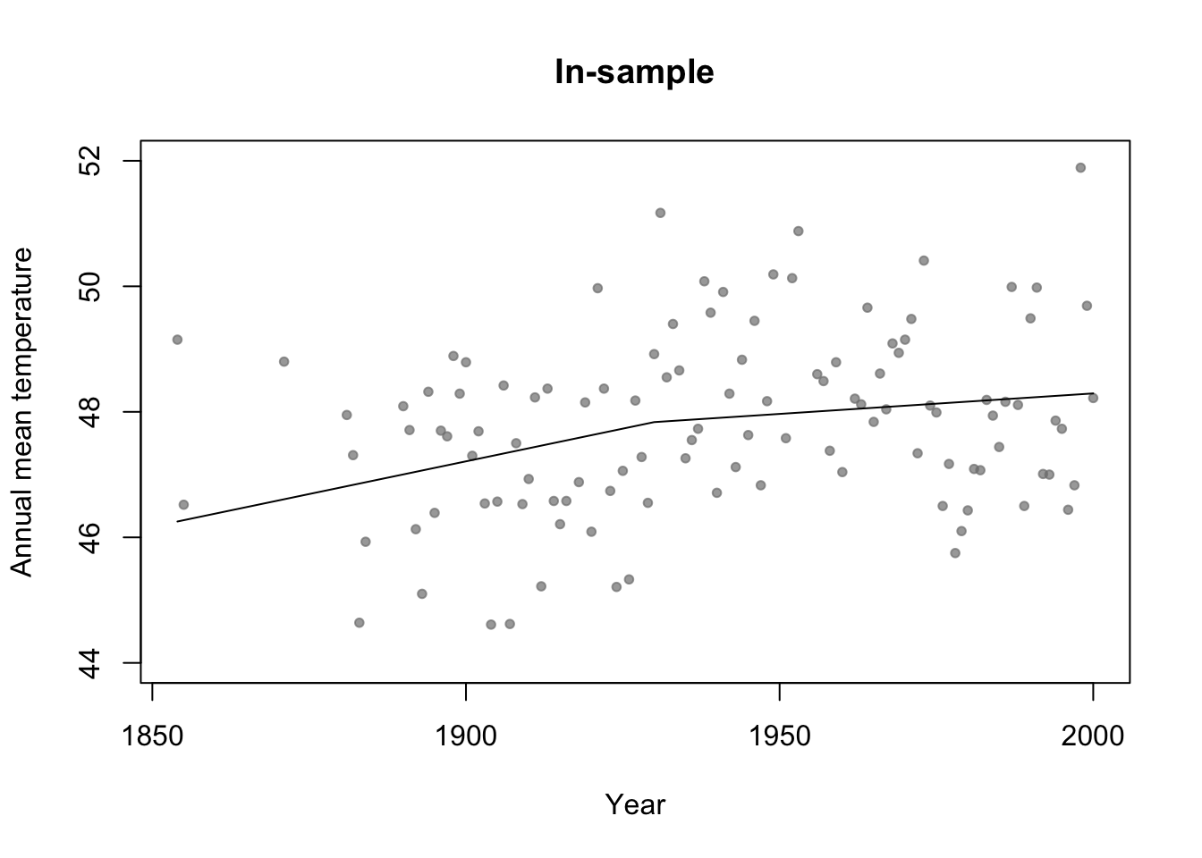
library(rpart)
# Fit regression tree model
m4 <- rpart(temp ~ year,data=df.in_sample)

par(mfrow=c(1,1))
# Plot predictions (in-sample)
plot(df.in_sample$year,df.in_sample$temp,main="In-sample",xlab="Year",ylab="Annual mean temperature",ylim=c(44,52),pch=20,col=rgb(0.5,0.5,0.5,0.7))
lines(df.in_sample$year,predict(m4))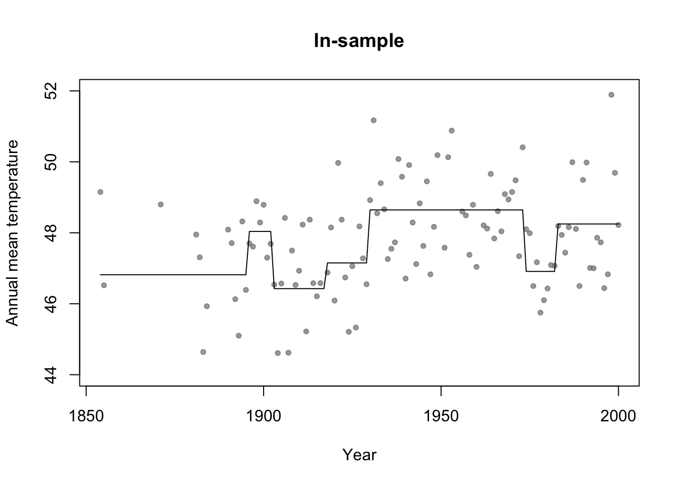
#Adjusted R-squared
summary(m1)$adj.r.square
## [1] 0summary(m2)$adj.r.square## [1] 0.0772653summary(m3)$adj.r.square## [1] 0.07692598# Not clear how to calculate adjusted R^2 for m4 (regression tree) # AIC y <- df.in_sample$temp y.hat_m1 <- predict(m1,newdata=df.in_sample) y.hat_m2 <- predict(m2,newdata=df.in_sample) y.hat_m3 <- predict(m3,newdata=df.in_sample) y.hat_m4 <- predict(m4,newdata=df.in_sample) sigma2.hat_m1 <- summary(m1)$sigma^2 sigma2.hat_m2 <- summary(m2)$sigma^2 sigma2.hat_m3 <- summary(m3)$sigma^2 # m1 #log-likelihood ll <- sum(dnorm(y,y.hat_m1,sigma2.hat_m1^0.5,log=TRUE)) # same as logLik(m1) q <- 1 + 1 # number of estimated betas + number estimated sigma2s #AIC -2*ll+2*q #Same as AIC(m1)## [1] 426.6276# m2 #log-likelihood ll <- sum(dnorm(y,y.hat_m2,sigma2.hat_m2^0.5,log=TRUE)) # same as logLik(m2) q <- 2 + 1 # number of estimated betas + number estimated sigma2s #AIC -2*ll+2*q #Same as AIC(m2)## [1] 418.38# m3 #log-likelihood ll <- sum(dnorm(y,y.hat_m3,sigma2.hat_m3^0.5,log=TRUE)) # same as logLik(m3) q <- 3 + 1 # number of estimated betas + number estimated sigma2s #AIC -2*ll+2*q #Same as AIC(m3)## [1] 419.4223# m4 n <- length(y) q <- 7 + 6 + 1 # number of estimated "intercept" terms in each termimal node + number of estimated "breaks" + number estimated sigma2s sigma2.hat_m4 <- t(y - y.hat_m4)%*%(y - y.hat_m4)/(n - q - 1) # log-likelihood ll <- sum(dnorm(y,y.hat_m4,sigma2.hat_m4^0.5,log=TRUE)) #AIC -2*ll+2*q## [1] 406.5715Example: assessing uncertainity in model selection statistics
library(mosaic)

boot <- function(){
m1 <- lm(temp ~ 1,data=resample(df.in_sample))
m2 <- lm(temp ~ year,data=resample(df.in_sample))
m3 <- lm(temp ~ f1(year,1930) + f2(year,1930),data=resample(df.in_sample))
cbind(AIC(m1),AIC(m2),AIC(m3))}

bs.aic.samplles <- do(1000)*boot()

par(mfrow=c(3,1))
hist(bs.aic.samplles[,1],col="grey",main="m1",freq=FALSE,xlab="AIC score",xlim=range(bs.aic.samplles))
abline(v=AIC(m1),col="gold",lwd=3)
hist(bs.aic.samplles[,2],col="grey",main="m2",freq=FALSE,xlab="AIC score",xlim=range(bs.aic.samplles))
abline(v=AIC(m2),col="gold",lwd=2)
hist(bs.aic.samplles[,3],col="grey",main="m3",freq=FALSE,xlab="AIC score",xlim=range(bs.aic.samplles))
abline(v=AIC(m3),col="gold",lwd=3)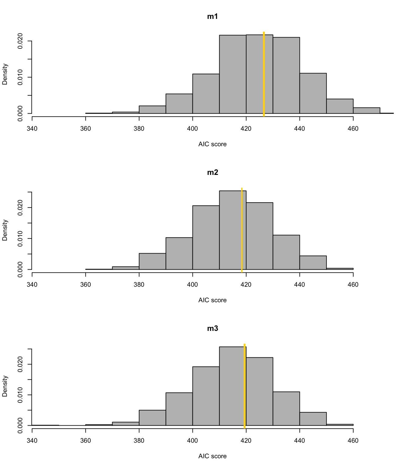
Summary
- Making statistical inference after model selection?
- Discipline specific views (e.g., AIC in wildlife ecology).
- There are many choices for model selection using in-sample data. Knowing the “best” model selection approach would require you to know a lot about all other procedures.
- AIC (Akaike 1973)
- BIC (Swartz 1978)
- CAIC (Vaida & Blanchard 2005)
- DIC (Spiegelhalter et al. 2002)
- ERIC (Hui et al. 2015)
- And the list goes on
- I would recommend using methods that you understand.
- In my experience it takes a larger data set to do estimation and model selection
- If you have a large data set, split it and use out-of-sample data for estimation
- If you don’t have a large data set, make sure you assess the uncertainty. You might not have enough data to do both estimation and model selection.
References
Faraway, J. J. 2014. Linear Models with r. CRC Press.
Gelman, Andrew, Jessica Hwang, and Aki Vehtari. 2014. “Understanding Predictive Information Criteria for Bayesian Models.” Statistics and Computing 24 (6): 997–1016.