10 Day 10 (June 16)

10.1 Announcements

• Read Ch. 3 in linear models with R

10.2 Maximum Likelihood Estimation

• Maximum likelihood estimation for the linear model
  • Assume that $\mathbf{y}\sim \text{N}(\mathbf{X}\boldsymbol{\beta},\sigma^2\mathbf{I})$
  • Write out the likelihood function $$\mathcal{L}(\boldsymbol{\beta},\sigma^2)=\prod_{i=1}^n\frac{1}{\sqrt{2\pi\sigma^2}}\textit{e}^{-\frac{1}{2\sigma^2}(y_{i} - \mathbf{x}_{i}^{\prime}\boldsymbol{\beta})^2}.$$
  • Maximize the likelihood function
    1. First take the natural log of $\mathcal{L}(\boldsymbol{\beta},\sigma^2)$, which gives $$\mathcal{l}(\boldsymbol{\beta},\sigma^2)=-\frac{n}{2}\text{ log}(2\pi\sigma^2) - \frac{1}{2\sigma^2}\sum_{i=1}^{n}(y_{i} - \mathbf{x}_{i}^{\prime}\boldsymbol{\beta})^2.$$
    2. Recall that $\sum_{i=1}^{n}(y_{i} - \mathbf{x}_{i}^{\prime}\boldsymbol{\beta})^2 = (\mathbf{y} - \mathbf{X}\boldsymbol{\beta})^{\prime}(\mathbf{y} - \mathbf{X}\boldsymbol{\beta})$
    3. Maximize the log-likelihood function $$\underset{\boldsymbol{\beta}, \sigma^2}{\operatorname{argmax}} -\frac{n}{2}\text{ log}(2\pi\sigma^2) - \frac{1}{2\sigma^2}(\mathbf{y} - \mathbf{X}\boldsymbol{\beta})^{\prime}(\mathbf{y} - \mathbf{X}\boldsymbol{\beta})$$
  • Visual for data $\mathbf{y}=(0.16,2.82,2.24)'$ and $\mathbf{x}=(1,2,3)'$
• Three ways to do it in program R
  • Using matrix calculus and algebra

  # Data 
  y <- c(0.16,2.82,2.24)
  X <- matrix(c(1,1,1,1,2,3),nrow=3,ncol=2,byrow=FALSE)
  n <- length(y)
  
  # Maximum likelihood estimation using closed from estimators
  beta <- solve(t(X)%*%X)%*%t(X)%*%y 
  sigma2 <- (1/n)*t(y-X%*%beta)%*%(y-X%*%beta)
  
  beta

  ##       [,1]
  ## [1,] -0.34
  ## [2,]  1.04

  sigma2

  ##        [,1]
  ## [1,] 0.5832

  • Using modern (circa 1970’s) optimization techniques

  # Maximum likelihood estimation estimation using Nelder-Mead algorithm
  y <- c(0.16,2.82,2.24)
  X <- matrix(c(1,1,1,1,2,3),nrow=3,ncol=2,byrow=FALSE)
  
  negloglik <- function(par){
  beta <- par[1:2]
  sigma2 <- par[3]
  -sum(dnorm(y,X%*%beta,sqrt(sigma2),log=TRUE))
  }
  optim(par=c(0,0,1),fn=negloglik,method = "Nelder-Mead")

  ## $par
  ## [1] -0.3397162  1.0398552  0.5831210
  ## 
  ## $value
  ## [1] 3.447978
  ## 
  ## $counts
  ## function gradient 
  ##      150       NA 
  ## 
  ## $convergence
  ## [1] 0
  ## 
  ## $message
  ## NULL

  • Using modern and user friendly statistical computing software

  # Maximum likelihood estimation using lm function
  # Note: estimate of sigma2 is not the MLE! 
  df <- data.frame(y = c(0.16,2.82,2.24),x = c(1,2,3))
  m1 <- lm(y~x,data=df)
  
  coef(m1)

  ## (Intercept)           x 
  ##       -0.34        1.04

  summary(m1)$sigma^2

  ## [1] 1.7496

  summary(m1)

  ## 
  ## Call:
  ## lm(formula = y ~ x, data = df)
  ## 
  ## Residuals:
  ##     1     2     3 
  ## -0.54  1.08 -0.54 
  ## 
  ## Coefficients:
  ##             Estimate Std. Error t value Pr(>|t|)
  ## (Intercept)  -0.3400     2.0205  -0.168    0.894
  ## x             1.0400     0.9353   1.112    0.466
  ## 
  ## Residual standard error: 1.323 on 1 degrees of freedom
  ## Multiple R-squared:  0.5529, Adjusted R-squared:  0.1057 
  ## F-statistic: 1.236 on 1 and 1 DF,  p-value: 0.4663

• Live example
  • Research publication
  • Data
  • R Script

10.3 Confidence intervals for paramters

• Example

  • Northern bobwhite quail

  y <- c(63, 68, 61, 44, 103, 90, 107, 105, 76, 46, 60, 66, 58, 39, 64, 29, 37,
  27, 38, 14, 38, 52, 84, 112, 112, 97, 131, 168, 70, 91, 52, 33, 33, 27,
  18, 14, 5, 22, 31, 23, 14, 18, 23, 27, 44, 18, 19)
  year <- 1965:2011
  df <- data.frame(y = y, year = year)
  plot(x = df$year, y = df$y, xlab = "Year", ylab = "Annual count", main = "",
  col = "brown", pch = 20, xlim = c(1965, 2040))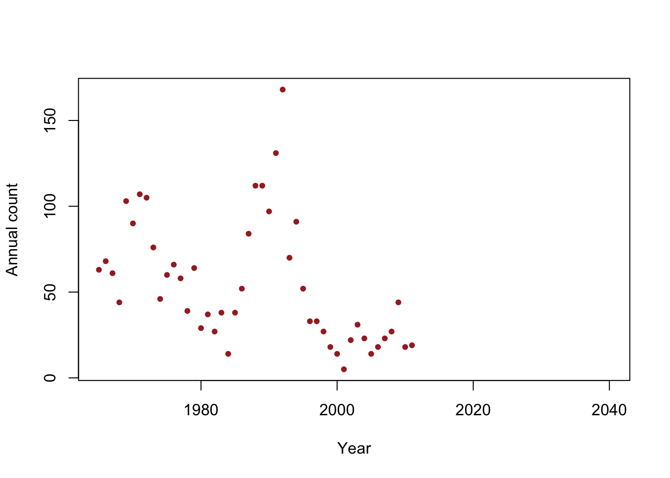

  

  • Is the population size really decreasing?
  • Write out the model we should use answer this question
  • How can we assess the uncertainty in our estimate of $\beta_1$?
  • Confidence intervals in R

  m1 <- lm(y~year,data=df)
  coef(m1)

  ## (Intercept)        year 
  ##  2356.48797    -1.15784

  confint(m1,level=0.95)    

  ##                 2.5 %       97.5 %
  ## (Intercept) 929.80699 3783.1689540
  ## year         -1.87547   -0.4402103

  • Note $$\hat{\boldsymbol{\beta}}\sim\text{N}(\boldsymbol{\beta},\sigma^2(\mathbf{X}^{\prime}\mathbf{X})^{-1})$$ and let $$\hat{\beta_1}\sim\text{N}(\beta_1,\sigma^{2}_{\beta_1})$$ where $\sigma^{2}_{\beta_1}= \sigma^2\mathbf{c}^{\prime}(\mathbf{X}^{\prime}\mathbf{X})^{-1}\mathbf{c}$ and $\mathbf{c}\equiv(0,1,0,0,\ldots,0)^{\prime}$. In R we can extract $\sigma^2(\mathbf{X}^{\prime}\mathbf{X})^{-1}$ using vcov().

  vcov(m1)  

  ##             (Intercept)         year
  ## (Intercept) 501753.2825 -252.3792372
  ## year          -252.3792    0.1269513

  Note that

  diag(vcov(m1))^0.5

  ## (Intercept)        year 
  ## 708.3454542   0.3563023

  corresponds to the column Std. Error from summary()

  summary(m1)

  ## 
  ## Call:
  ## lm(formula = y ~ year, data = df)
  ## 
  ## Residuals:
  ##     Min      1Q  Median      3Q     Max 
  ## -45.333 -20.597  -9.754  14.035 117.929 
  ## 
  ## Coefficients:
  ##              Estimate Std. Error t value Pr(>|t|)   
  ## (Intercept) 2356.4880   708.3455   3.327  0.00176 **
  ## year          -1.1578     0.3563  -3.250  0.00219 **
  ## ---
  ## Signif. codes:  0 '***' 0.001 '**' 0.01 '*' 0.05 '.' 0.1 ' ' 1
  ## 
  ## Residual standard error: 33.13 on 45 degrees of freedom
  ## Multiple R-squared:  0.1901, Adjusted R-squared:  0.1721 
  ## F-statistic: 10.56 on 1 and 45 DF,  p-value: 0.00219

  • When $\sigma_{\beta_1}$ is known $$\hat{\beta_1}\sim\text{N}(\beta_1,\sigma^{2}_{\beta_1})$$ $$\hat{\beta_1} - \beta_1 \sim\text{N}(0,\sigma^{2}_{\beta_1})$$ $$\frac{\hat{\beta_1} - \beta_1}{\sigma_{\beta_1}} \sim\text{N}(0,1)$$
  • When $\sigma_{\beta_1}$ is estimated $$\frac{\hat{\beta_1} - \beta_1}{\hat{\sigma}_{\beta_1}} \sim\text{t}(\nu)$$ where $\nu = n - p$
  • Deriving the confidence interval for $\hat{\beta_1}$ $$\text{P}(a < \frac{\hat{\beta_1} - \beta_1}{\hat{\sigma}_{\beta_1}} < b) = 1-\alpha$$ $$\text{P}(a\hat{\sigma}_{\beta_1} < \hat{\beta_1} - \beta_1 < b\hat{\sigma}_{\beta_1}) = 1-\alpha$$ $$\text{P}(-\hat{\beta_1} + a\hat{\sigma}_{\beta_1} < - \beta_1 < -\hat{\beta_1} + b\hat{\sigma}_{\beta_1}) = 1-\alpha$$ $$\text{P}(\hat{\beta_1} - b\hat{\sigma}_{\beta_1} < \beta_1 < \hat{\beta_1} - a\hat{\sigma}_{\beta_1}) = 1-\alpha$$
  • What is $\text{P}(a < \frac{\hat{\beta_1} - \beta_1}{\hat{\sigma}_{\beta_1}} < b) = 1-\alpha$? $$\text{P}(a < z < b) = \int_{a}^{b}[z|\nu]dz$$
  • “By hand” in R

  nu <- length(df$y) - 2
  a <- qt(p = 0.025,df = nu)
  a

  ## [1] -2.014103

  b <- qt(p = 0.975,df = nu)
  b

  ## [1] 2.014103

  beta1.hat <- coef(m1)[2]
  sigma.beta1.hat <- (diag(vcov(m1))^0.5)[2]
  
  beta1.hat - b*sigma.beta1.hat

  ##     year 
  ## -1.87547

  beta1.hat - a*sigma.beta1.hat

  ##       year 
  ## -0.4402103

  confint(m1)[2,]

  ##      2.5 %     97.5 % 
  ## -1.8754696 -0.4402103