35 Day 35 (July 25)
35.2 Generalized linear models
The generalized linear model framework \[\mathbf{y} \sim[\mathbf{\mathbf{y}|\boldsymbol{\mu},\psi]}\] \[g(\boldsymbol{\mu})=\mathbf{X}\boldsymbol{\beta}\]
- \([\mathbf{y}|\boldsymbol{\mu},\psi]\) is a distribution from the exponential family (e.g., normal, Poisson, binomial) with expected value \(\boldsymbol{\mu}\) and dispersion parameter \(\psi\).
- Example \([\mathbf{y}|\boldsymbol{\mu},\psi]=\text{N}\left(\boldsymbol{\mu},\psi\mathbf{I}\right)\)
- Example \([\mathbf{\mathbf{y}|\boldsymbol{\mu},\psi]}=\text{Poisson}\left(\boldsymbol{\mu}\right)\)
- Example \([\mathbf{\mathbf{y}|\boldsymbol{\mu},\psi]}=\text{gamma}\left(\boldsymbol{\mu},\psi\right)\)
- \([\mathbf{y}|\boldsymbol{\mu},\psi]\) is a distribution from the exponential family (e.g., normal, Poisson, binomial) with expected value \(\boldsymbol{\mu}\) and dispersion parameter \(\psi\).
Estimation
- Use numerical maximization to estimate
- \(\hat{\boldsymbol{\beta}}=(\mathbf{X}^{\prime}\mathbf{X})^{-1}\mathbf{X}^{\prime}\mathbf{y}\) is NOT the MLE for the glm
- Inference is based on asymptotic properties of MLE.
- Example: Challenger data
- The statistical model: \[\mathbf{y}\sim\text{binomial}(6,\mathbf{p})\] \[\text{logit}(\mathbf{p})=\mathbf{X}\boldsymbol{\beta}.\]
- The PMF for the binomial distribution \[\binom{N}{y}p^{y}(1-p)^{N-y}\]
- Write out the likelihood function \[\mathcal{L}(\boldsymbol{\beta})=\prod_{i=1}^n\binom{6}{y_i}p_i^{y_i}(1-p_i)^{6-y_i}\]
- Maximize the log-likelihood function
challenger <- read.csv("https://www.dropbox.com/s/ezxj8d48uh7lzhr/challenger.csv?dl=1")


y <- challenger$O.ring
X <- model.matrix(~Temp,data= challenger)

nll <- function(beta){
  p <- 1/(1+exp(-X%*%beta)) # Inverse of logit link function
  -sum(dbinom(y,6,p,log=TRUE)) # Sum of the log likelihood for each observation
  }
est <- optim(par=c(0,0),fn=nll,hessian=TRUE)

# MLE of beta
est$par
## [1] 6.751192 -0.139703# Var(beta.hat) diag(solve(est$hessian))## [1] 8.830866683 0.002145791# Std.Error diag(solve(est$hessian))^0.5## [1] 2.97167742 0.04632268- Using the
glm()function
m1 <- glm(cbind(challenger$O.ring,6-challenger$O.ring) ~ Temp, family = binomial(link = "logit"),data=challenger)
summary(m1)
## ## Call: ## glm(formula = cbind(challenger$O.ring, 6 - challenger$O.ring) ~ ## Temp, family = binomial(link = "logit"), data = challenger) ## ## Deviance Residuals: ## Min 1Q Median 3Q Max ## -0.9876 -0.7798 -0.4987 -0.2975 2.7483 ## ## Coefficients: ## Estimate Std. Error z value Pr(>|z|) ## (Intercept) 6.75183 2.97989 2.266 0.02346 * ## Temp -0.13971 0.04647 -3.007 0.00264 ** ## --- ## Signif. codes: 0 '***' 0.001 '**' 0.01 '*' 0.05 '.' 0.1 ' ' 1 ## ## (Dispersion parameter for binomial family taken to be 1) ## ## Null deviance: 28.761 on 22 degrees of freedom ## Residual deviance: 19.093 on 21 degrees of freedom ## AIC: 36.757 ## ## Number of Fisher Scoring iterations: 5- Prediction
- We can get prediction using \(\mathbf{X}\hat{\boldsymbol{\beta}}\) or the inverse of the logit link function \(\hat{\boldsymbol{\mu}}=\frac{1}{1+e^{-\mathbf{X}\hat{\boldsymbol{\beta}}}}\)
- Confidence intervals for \(\mathbf{X}\hat{\boldsymbol{\beta}}\) are straightforward
- Confidence intervals for \(\hat{\boldsymbol{\mu}}=\frac{1}{1+e^{-\mathbf{X}\hat{\boldsymbol{\beta}}}}\) are not straightforward because of the nonlinear transformation of \(\hat{\boldsymbol{\beta}}\)
beta.hat <- coef(m1)

new.temp <- seq(0,80,by=0.01)
X.new <- model.matrix(~new.temp)

mu.hat <- (1/(1+exp(-X.new%*%beta.hat)))

plot(challenger$Temp,challenger$O.ring,xlab="Temperature",ylab="Number of incidents",xlim=c(10,80),ylim=c(0,6))
points(new.temp,6*mu.hat,typ="l",col="red")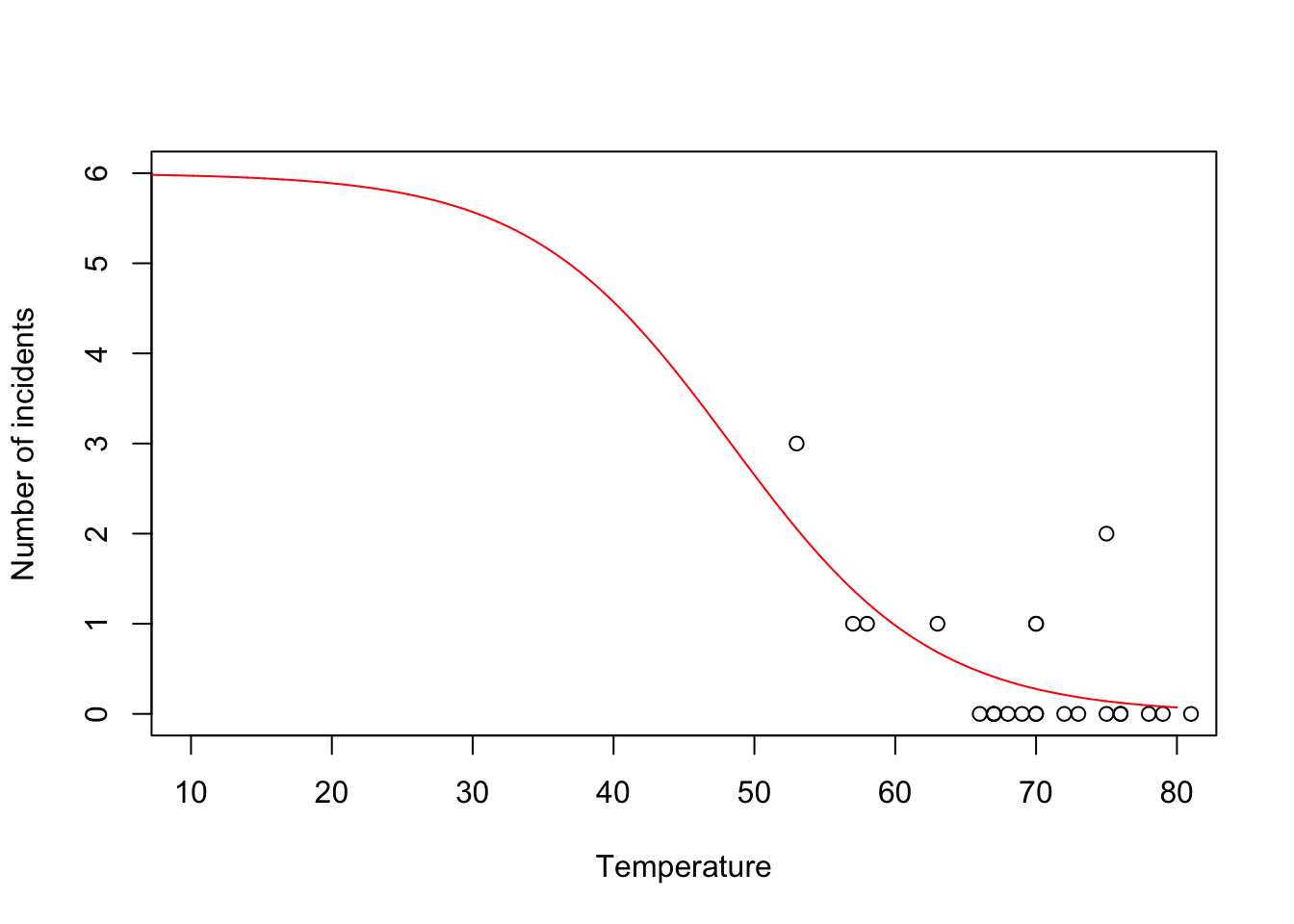
- Predictive distribution
library(mosaic)

predict.bs <- function(){
  m1 <- glm(cbind(O.ring,6-O.ring) ~ Temp, family = binomial(link = "logit"),data=resample(challenger))
  p <- predict(m1,newdata=data.frame(Temp=31),type="response")
  y <- rbinom(1,6,p)
  y
}

bootstrap <- do(1000)*predict.bs()

par(mar = c(5, 4, 7, 2))
hist(bootstrap[,1], col = "grey", xlab = "Year", main = "Empirical distribution of O-ring failures at 31 degrees", freq = FALSE,right=FALSE,breaks=c(-0.5:6.5))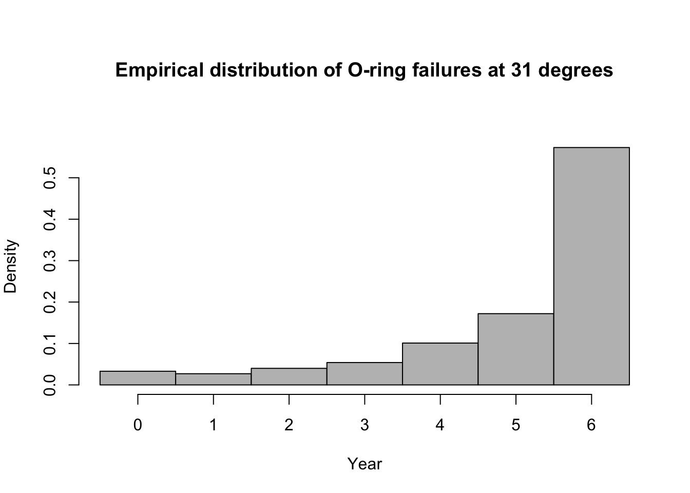
# 95% equal-tailed CI based on percentiles of the empirical distribution
quantile(bootstrap[,1], prob = c(0.025, 0.975))
## 2.5% 97.5% ## 0 6# Proability of 6 O-rings failing length(which(bootstrap[,1]==6))/dim(bootstrap)[1]## [1] 0.573Summary
- The generalized linear model useful when the distributional assumptions of linear model are untenable.
- Small counts
- Binary data
- Two cultures
- All distributions are approximations of a unknown data generating process so why does it matter? Use the linear model because it is easier to understand.
- Personal philosophy
- Picking a distribution whose support matches that of the data gets closer to the etiology of the process that generated the data.
- Easier for me to think scientifically about the process
- The generalized linear model useful when the distributional assumptions of linear model are untenable.