28 Day 28 (July 14)
28.1 Announcements
Work days next tuesday and thursday
Guide and opportunity for improvement for assignment 3 is available
Assignment 4 is posted and due next Friday
Presentations will occur between Monday July 24 - Friday July 28.
Please email me to request a 20-30 min time slot between 10:30 am and 4 pm to give your final presentation. When you email me, please give 3 dates/time that work for you.
Short example related to question about factors (R code)
28.2 Constant variance
If \(\mathbf{y}\sim\text{N}(\mathbf{X\boldsymbol{\beta}},\sigma^{2}\mathbf{I})\), then each \(\varepsilon_i\) follows a normal distribution with the same value of \(\sigma^2\).
- A linear model with constant variance is the simplest possible model we could assume. It is like the intercept only model in that regard.
- Example: Hubble data
library(gamair)
data(hubble)

m1 <- lm(y ~ x - 1, data = hubble)
confint(m1)
## 2.5 % 97.5 % ## x 68.37937 84.78297# Plot data and E(y) plot(hubble$x,hubble$y,xlab="Distance (Mpc)", ylab=expression("Velocity (km"*s^{-1}*")"),pch=20) abline(m1)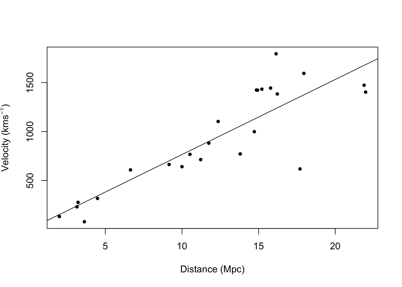
# Plot residuals vs. x
e.hat <- residuals(m1)
hist(e.hat,col="grey",breaks=15,main="",xlab=expression(hat(epsilon)))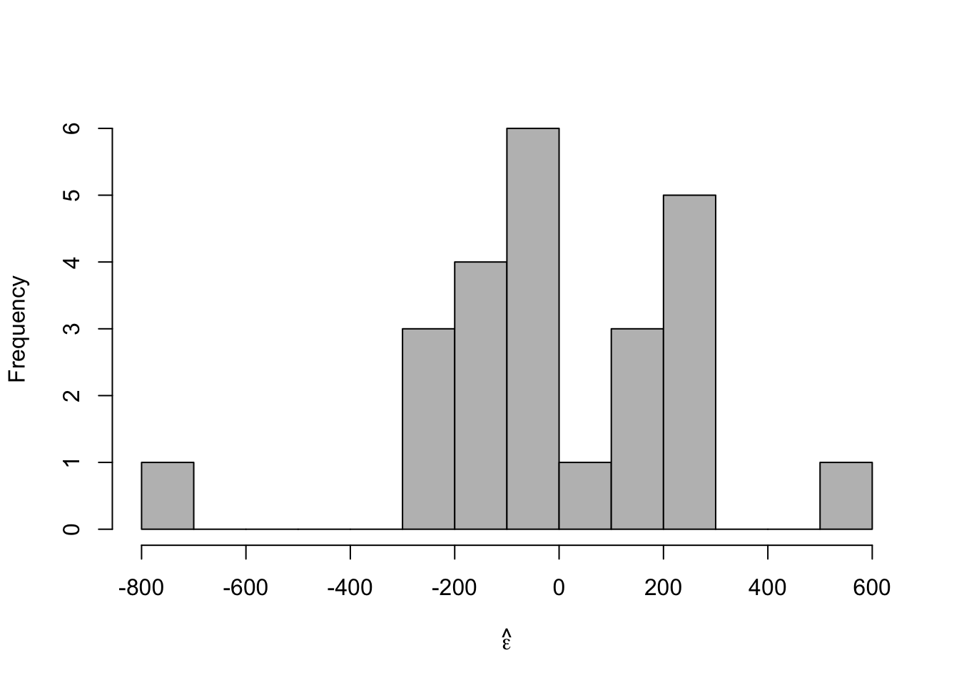
plot(hubble$x,e.hat,xlab="Distance(Mpc)",ylab=expression(hat(epsilon)),pch=20)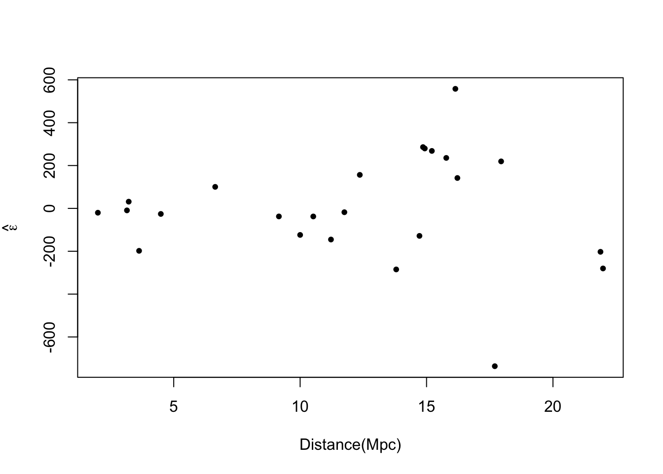
# Plot prediction intervals
y.pi <- predict(m1,newdata=data.frame(x = 0:25),interval = "predict")
plot(hubble$x,hubble$y,xlab="Distance (Mpc)",
ylab=expression("Velocity (km"*s^{-1}*")"),xlim=c(0,25),ylim=c(0,2500),pch=20)
points(0:25,y.pi[,2],typ="l",lwd=2,col="purple")
points(0:25,y.pi[,3],typ="l",lwd=2,col="purple")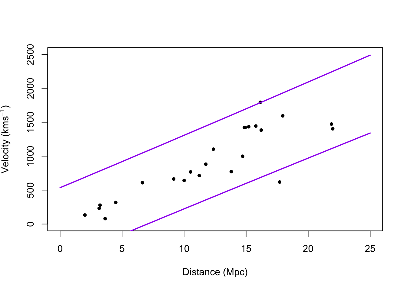
- A test for equal variance (see pg. 77 in Faraway (2014))
- What causes non-constant variance (also called heteroskedasticity).
What can be done?
- A transformation may work (see pg. 77 Faraway (2014))
- Build a more appropriate model for the variance. For example, \[\mathbf{y}\sim\text{N}(\mathbf{X\boldsymbol{\beta}},\mathbf{V})\] where the \(i^\text{th}\) and \(j^{th}\) entry of the matrix \(\mathbf{V}\) equals \[v_{ij}(\theta)=\begin{cases} \sigma^{2}e^{2\theta x_i} &\text{if}\ i=j\\ 0 &\text{if}\ i\neq j \end{cases}\]
library(nlme)
m2 <- gls(y~x-1,weights = varExp(form=~x),data=hubble)
summary(m2)
## Generalized least squares fit by REML ## Model: y ~ x - 1 ## Data: hubble ## AIC BIC logLik ## 322.432 325.8385 -158.216 ## ## Variance function: ## Structure: Exponential of variance covariate ## Formula: ~x ## Parameter estimates: ## expon ## 0.1060336 ## ## Coefficients: ## Value Std.Error t-value p-value ## x 76.2548 3.854585 19.78288 0 ## ## Standardized residuals: ## Min Q1 Med Q3 Max ## -2.4272668 -0.4726915 -0.1548023 0.7929118 1.8437320 ## ## Residual standard error: 55.17695 ## Degrees of freedom: 24 total; 23 residualconfint(m2)## 2.5 % 97.5 % ## x 68.69995 83.80965# Plot prediction intervals X <- model.matrix(y~x-1,data=hubble) sigma2.hat <- summary(m1)$sigma^2 sigma2.hat*solve(t(X)%*%X)## x ## x 15.71959vcov(m1)## x ## x 15.71959X <- model.matrix(y~x-1,data=hubble) beta.hat <- coef(m2) sigma2.hat <- summary(m2)$sigma^2 theta.hat <- summary(m2)$modelStruct$varStruct V <- diag(c(sigma2.hat*exp(2*X%*%theta.hat))) X.new <- model.matrix(~x-1,data=data.frame(x = 1:25)) y.pi <- cbind(X.new%*%beta.hat - qt(0.975,24-1)*sqrt(X.new^2%*%solve(t(X)%*%solve(V)%*%X) + sigma2.hat*exp(2*X.new%*%theta.hat)), X.new%*%beta.hat + qt(0.975,24-1)*sqrt(X.new^2%*%solve(t(X)%*%solve(V)%*%X) + sigma2.hat*exp(2*X.new%*%theta.hat))) plot(hubble$x,hubble$y,xlab="Distance (Mpc)", ylab=expression("Velocity (km"*s^{-1}*")"),xlim=c(0,25),ylim=c(0,2500),pch=20) points(1:25,y.pi[,1],typ="l",lwd=2,col="purple") points(1:25,y.pi[,2],typ="l",lwd=2,col="purple")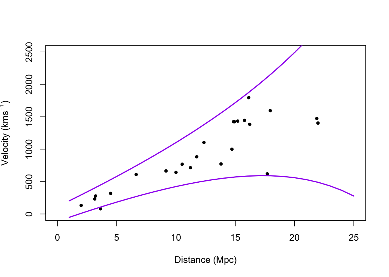
- Example: Schizophrenia data
url <- "http://www.stat.columbia.edu/~gelman/book/data/schiz.asc"
df1 <- data.frame(time = scan(url,skip=5),schizophrenia = c(rep("no",30*11),rep("yes",30*6)))
head(df1)
## time schizophrenia ## 1 312 no ## 2 272 no ## 3 350 no ## 4 286 no ## 5 268 no ## 6 328 noboxplot(time~schizophrenia,data=df1,xlab = "Schizophrenic",ylab="Reaction time (in milliseconds)")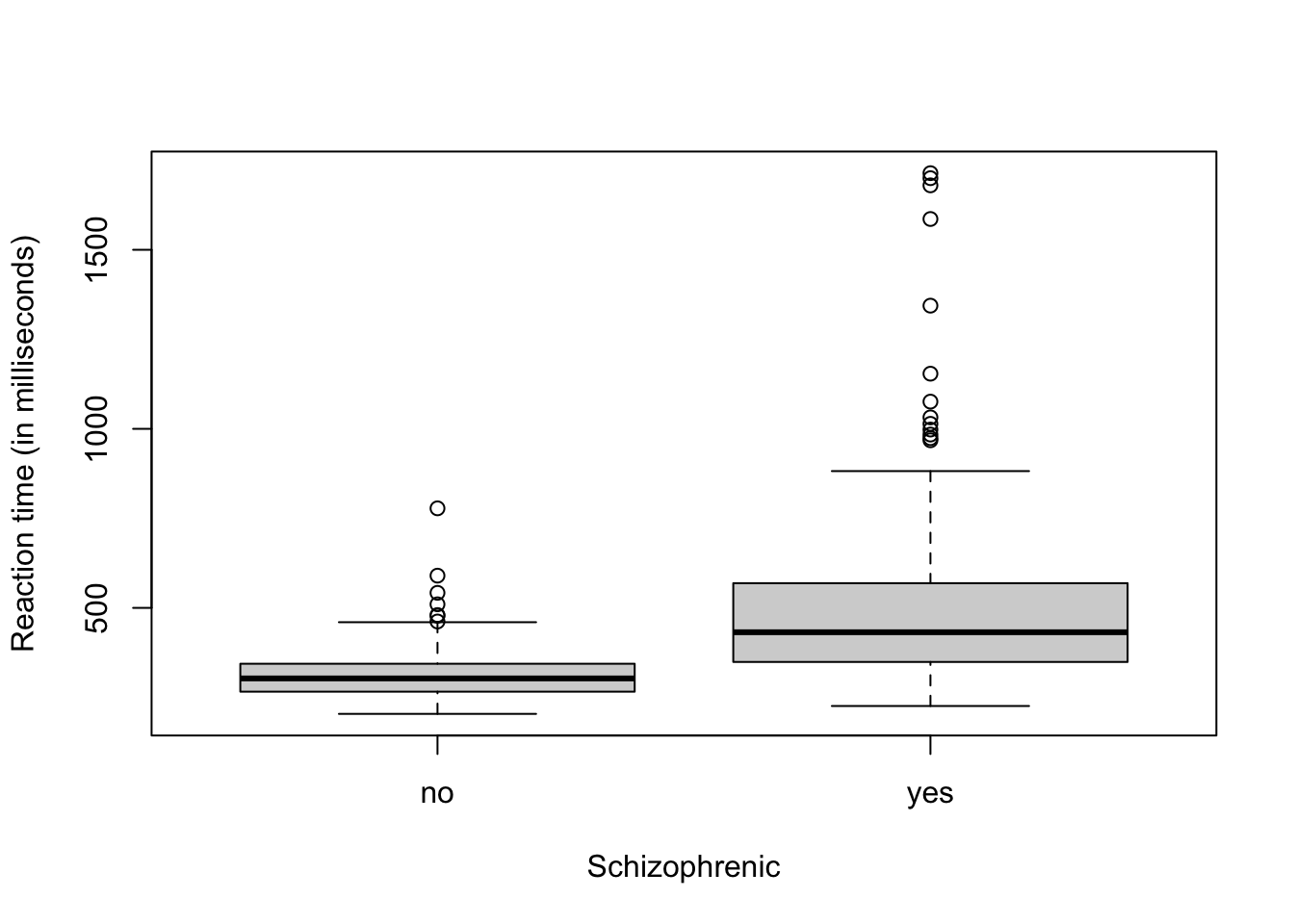
Example
- Linear model with constant variance
m1 <- lm(time ~ schizophrenia,data=df1)
summary(m1)
## ## Call: ## lm(formula = time ~ schizophrenia, data = df1) ## ## Residuals: ## Min 1Q Median 3Q Max ## -280.87 -70.17 -16.52 37.66 1207.13 ## ## Coefficients: ## Estimate Std. Error t value Pr(>|t|) ## (Intercept) 310.170 9.057 34.25 <2e-16 *** ## schizophreniayes 196.697 15.245 12.90 <2e-16 *** ## --- ## Signif. codes: 0 '***' 0.001 '**' 0.01 '*' 0.05 '.' 0.1 ' ' 1 ## ## Residual standard error: 164.5 on 508 degrees of freedom ## Multiple R-squared: 0.2468, Adjusted R-squared: 0.2453 ## F-statistic: 166.5 on 1 and 508 DF, p-value: < 2.2e-16- Plot residuals vs. predictor to check assumptions
e.hat <- residuals(m1)
x <- model.matrix(m1)[,2]
plot(x,e.hat,ylab=expression(hat(epsilon)))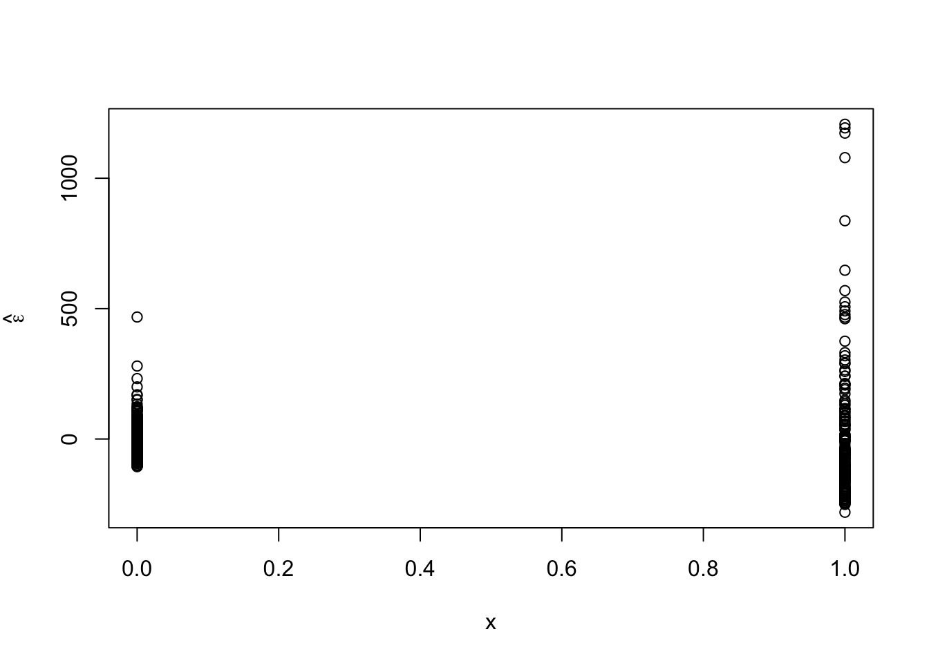
- Plot residuals for each category
par(mfrow=c(2,1))
hist(e.hat[which(x==0)],col="grey",xlab=expression(hat(epsilon)),main=expression(hat(epsilon)*" for x = 0"),xlim=c(range(e.hat)),breaks=seq(min(e.hat),max(e.hat),length.out=40))
hist(e.hat[which(x==1)],col="grey",xlab=expression(hat(epsilon)),main=expression(hat(epsilon)*" for x = 1"),xlim=c(range(e.hat)),breaks=seq(min(e.hat),max(e.hat),length.out=40))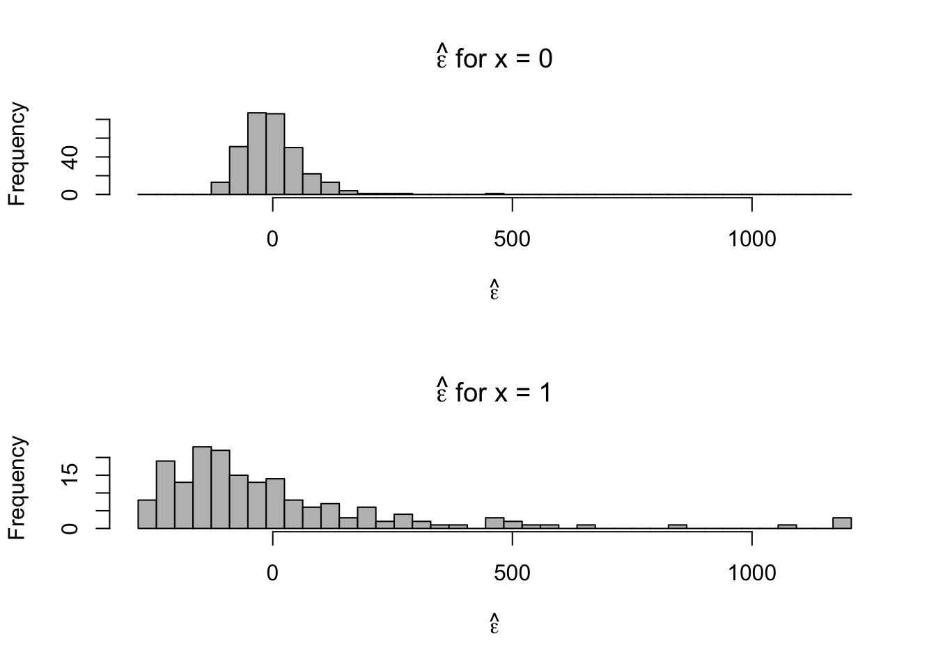
- Looks like there are some outliers due to skewness in the distribution of \(\mathbf{y}\) and the variance is not constant. Let’s tackle the problem of non-constant variance first.
- Some possible solutions
- Build a more appropriate model for the variance. For example, \[\mathbf{y}\sim\text{N}(\mathbf{X\boldsymbol{\beta}},\mathbf{V})\] where the \(i^\text{th}\) and \(j^{th}\) entry of the matrix \(\mathbf{V}\) equals \[v_{ij}(\theta)=\begin{cases} \sigma^{2}e^{2\theta x_i} &\text{if}\ i=j\\ 0 &\text{if}\ i\neq j \end{cases}\]
- For additional options see
?varClassesafter loading the nlme package in R. - Fit model using
?glsfunction
library(nlme)
x <- ifelse(df1$schizophrenia=="no",0,1)
m2 <- gls(time ~ schizophrenia, weights = varExp(form =~x), method = "REML",data=df1)
summary(m2)
## Generalized least squares fit by REML ## Model: time ~ schizophrenia ## Data: df1 ## AIC BIC logLik ## 6200.793 6217.715 -3096.396 ## ## Variance function: ## Structure: Exponential of variance covariate ## Formula: ~x ## Parameter estimates: ## expon ## 1.399026 ## ## Coefficients: ## Value Std.Error t-value p-value ## (Intercept) 310.1697 3.571554 86.84447 0 ## schizophreniayes 196.6970 19.914372 9.87714 0 ## ## Correlation: ## (Intr) ## schizophreniayes -0.179 ## ## Standardized residuals: ## Min Q1 Med Q3 Max ## -1.6363885 -0.6461803 -0.1875710 0.4166345 7.2106463 ## ## Residual standard error: 64.8805 ## Degrees of freedom: 510 total; 508 residual# 95% CI for theta/2 intervals(m2)$varStruct## lower est. upper ## expon 1.270308 1.399026 1.527744 ## attr(,"label") ## [1] "Variance function:"# See ?varExp theta.hat <- m2$model[1]$varStruct*2 sigma2.hat <- summary(m2)$sigma^2 sigma2.hat*exp(theta.hat*0)## Variance function structure of class varExp representing ## expon ## 4209.479sigma2.hat*exp(theta.hat*1)## Variance function structure of class varExp representing ## expon ## 69088.72# Check compared to sample variance var(df1$time[which(df1$schizophrenia=="no")])## [1] 4209.479var(df1$time[which(df1$schizophrenia=="yes")])## [1] 69088.72# p-value from glm should be the same as t-test with unequal variances t.test(time ~ schizophrenia,alternative = c("two.sided"),mu = 0, var.equal = FALSE,data = df1)## ## Welch Two Sample t-test ## ## data: time by schizophrenia ## t = -9.8771, df = 190.98, p-value < 2.2e-16 ## alternative hypothesis: true difference in means between group no and group yes is not equal to 0 ## 95 percent confidence interval: ## -235.9773 -157.4166 ## sample estimates: ## mean in group no mean in group yes ## 310.1697 506.8667# Conclusiongs from var.test should match up with m2 var.test(time ~ schizophrenia,alternative = c("two.sided"),data = df1)## ## F test to compare two variances ## ## data: time by schizophrenia ## F = 0.060929, num df = 329, denom df = 179, p-value < 2.2e-16 ## alternative hypothesis: true ratio of variances is not equal to 1 ## 95 percent confidence interval: ## 0.04683408 0.07847916 ## sample estimates: ## ratio of variances ## 0.0609286- Plot residuals vs. predictor to check assumption
e.hat <- residuals(m2)
plot(x,e.hat,ylab=expression(hat(epsilon)))
- Plot residuals for each category
par(mfrow=c(2,1))
hist(e.hat[which(x==0)],col="grey",xlab=expression(hat(epsilon)),main=expression(hat(epsilon)*" for x = 0"),xlim=c(range(e.hat)),breaks=seq(min(e.hat),max(e.hat),length.out=40))
hist(e.hat[which(x==1)],col="grey",xlab=expression(hat(epsilon)),main=expression(hat(epsilon)*" for x = 1"),xlim=c(range(e.hat)),breaks=seq(min(e.hat),max(e.hat),length.out=40))
- Normal distribution is symmetric, the support of reaction times is always positive. We probably won’t be able to alleviate the issue of skewness using the normal distribution.
References
Faraway, J. J. 2014. Linear Models with r. CRC Press.