38 Day 36 (July 28)

38.1 Announcements

• Please fill out teaching evaluations!
• I will email you your final grade before I submitt anything

38.2 Data fusion

• Data fusion is a term used to describe a statistical model that uses more than one source of data.

  • A common situation is when we have responses variables (i.e., \(\mathbf{y}\)) from different studies or experiments.
  • Examples:
    • Age vs. height
    • Abundance vs. presence/absence
  • Other names include: data integration, data reconciliation, and multi-data source models

• Common approaches for modeling data from different sources or of different quality

  • Simple pooling
  • Don’t destroy/degrade good data!
  • Avoid non-invertible transformation to the response!
  • Example: Fletcher et al. (2019)

• General model building strategy

  • For each data source, pick an appropriate distribution for the response.
  • Select mathematical models that will be used to model the expected value (or other parameters such as the variance) of the distributions. The mathematical models may be the same for each distribution or may only share parameters.
  • Construct the likelihood function for each data source/statistical model.
  • Ideally the data sources are independent and, therefore, the likelihood function for each data source/statistical model can be multiplied
  • Proceed with estimation.

• Example: Konza percent grass cover

  • Exact cover data

  url <- "https://www.dropbox.com/scl/fi/g633b8ebwidskngmjf0vg/konza_grass_exact.csv?rlkey=y2ddh50ucyp92hwfwmi6lr2lj&dl=1"
  df.grass.exact <- read.csv(url)
  head(df.grass.exact)

  ##   percgrass    elev
  ## 1        13 420.860
  ## 2        45 399.306
  ## 3        72 412.792
  ## 4         9 422.606
  ## 5        21 381.152
  ## 6        37 397.789

  plot(df.grass.exact$elev,df.grass.exact$percgrass,xlab="Elevation",ylab="Percent grass")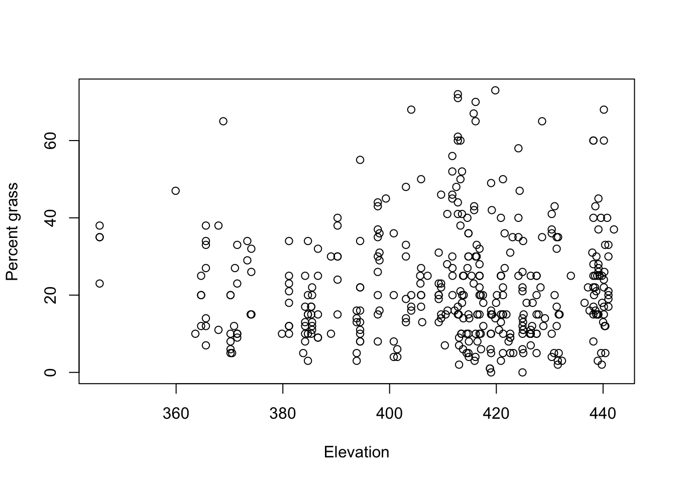

  

  m1 <- lm(percgrass~elev,df.grass.exact)
  summary(m1)

  ## 
  ## Call:
  ## lm(formula = percgrass ~ elev, data = df.grass.exact)
  ## 
  ## Residuals:
  ##     Min      1Q  Median      3Q     Max 
  ## -22.745 -10.850  -2.845   7.794  50.374 
  ## 
  ## Coefficients:
  ##             Estimate Std. Error t value Pr(>|t|)
  ## (Intercept) 12.86463   14.04673   0.916    0.360
  ## elev         0.02325    0.03416   0.681    0.496
  ## 
  ## Residual standard error: 14.84 on 398 degrees of freedom
  ## Multiple R-squared:  0.001163,   Adjusted R-squared:  -0.001347 
  ## F-statistic: 0.4633 on 1 and 398 DF,  p-value: 0.4965

  confint(m1)

  ##                    2.5 %      97.5 %
  ## (Intercept) -14.75042337 40.47968843
  ## elev         -0.04390688  0.09041252

  • Cheap cover data

  url <- "https://www.dropbox.com/scl/fi/gqigo9t23xlhhzuouta9f/konza_grass_cheap.csv?rlkey=jxbqo03fywky9g1lco336d17m&dl=1"
  df.grass.cheap <- read.csv(url)
  head(df.grass.cheap)

  ##   percgrass    elev
  ## 1      <50% 430.380
  ## 2      <50% 430.380
  ## 3      <50% 430.380
  ## 4      <50% 430.380
  ## 5      <50% 425.015
  ## 6      <50% 425.015

  • Model formulation (go over on white board)
  • Model implementation

  # Summary function for optim output (get maximum likelihood estimates, standard errors, and 95% CI )
  summary.opt <- function(est){round(data.frame(MLE = est$par,SE = diag(solve(est$hessian))^0.5,
                                            lower.CI = est$par-1.96*diag(solve(est$hessian))^0.5,
                                            upper.CI = est$par+1.96*diag(solve(est$hessian))^0.5),3)}
  
  # Perpare data
  X.y <- model.matrix(~elev,df.grass.exact)
  y <- df.grass.exact$percgrass
  X.z <- model.matrix(~elev,df.grass.cheap)
  z <- ifelse(df.grass.cheap$percgrass==">50%",1,0)
  
  # Negative log-likelihood function
  nll <- function(par){
    sigma2 <- exp(par[1])
    beta <- par[-1]
    -(sum(dnorm(y,X.y%*%beta,sqrt(sigma2),log=TRUE)) + sum(dbinom(z,1,pnorm(X.z%*%beta,50,sqrt(sigma2)),log=TRUE)))
  }
  
  # Obtain maximum likelihood estimates for beta and sigma2
  est <- optim(c(log(200),0,0),fn=nll,method="Nelder-Mead",hessian=TRUE)
  summary.opt(est)[2:3,]

  ##      MLE    SE lower.CI upper.CI
  ## 2 10.450 8.696   -6.595   27.494
  ## 3  0.031 0.021   -0.010    0.072

  # Compare 95% CI length for beta_1 from exact data only to data fusion
  (confint(m1)[2,2] - confint(m1)[2,1])/(summary.opt(est)[3,4] - summary.opt(est)[3,3])

  ## [1] 1.638041

• Summary

  • There are multiple ways to collect data on the same underlying phenomenon.
    • Some ways of collecting data are “better” than others, but there are many criteria to decide how to measure best.
    • Even if the data are collected using a standardized protocol it is a (testable) assumption that the error follows the same distribution for each observation.
  • The ability to build and combined statistical models for multiple types of data is becoming increasingly valuable.
    • Many ad hoc approaches exist (e.g., “correction factors” or “calibration”)
    • Unlikely to have easy to use software because of the large number of model combinations
    • Properties of such models are only beginning to be studied (e.g., optimal design)