4 Day 4 (June 8)

4.1 Announcements

• Intro resources for learning R and SAS

  • Stat 725 and 726

• If office hours times don’t work for you let me know

• Recommended reading

  • Chapters 1 and 2 (pgs 1 - 28) in Linear Models with R
  • Chapter 2 in Applied Regression and ANOVA Using SAS

4.2 Matrix algebra

• Column vectors
  • $\mathbf{y}\equiv(y_{1},y_{2},\ldots,y_{n})^{'}$
  • $\mathbf{x}\equiv(x_{1},x_{2},\ldots,x_{n})^{'}$
  • $\boldsymbol{\beta}\equiv(\beta_{1},\beta_{2},\ldots,\beta_{p})^{'}$
  • $\boldsymbol{1}\equiv(1,1,\ldots,1)^{'}$
  • In R

  y <- matrix(c(1,2,3),nrow=3,ncol=1)
  y

  ##      [,1]
  ## [1,]    1
  ## [2,]    2
  ## [3,]    3

• Matrices
  • $\mathbf{X}\equiv(\mathbf{x}_{1},\mathbf{x}_{2},\ldots,\mathbf{x}_{p})$
  • In R

  X <- matrix(c(1,2,3,4,5,6),nrow=3,ncol=2,byrow=FALSE)
  X

  ##      [,1] [,2]
  ## [1,]    1    4
  ## [2,]    2    5
  ## [3,]    3    6

• Vector multiplication
  • $\mathbf{y}^{'}\mathbf{y}$
  • $\mathbf{1}^{'}\mathbf{1}$
  • $\mathbf{1}\mathbf{1}^{'}$
  • In R

  t(y)%*%y    

  ##      [,1]
  ## [1,]   14

• Matrix by vector multiplication
  • $\mathbf{X}^{'}\mathbf{y}$
  • In R

  t(X)%*%y

  ##      [,1]
  ## [1,]   14
  ## [2,]   32

• Matrix by matrix multiplication
  • $\mathbf{X}^{'}\mathbf{X}$
  • In R

  t(X)%*%X

  ##      [,1] [,2]
  ## [1,]   14   32
  ## [2,]   32   77

• Matrix inversion
  • $(\mathbf{X}^{'}\mathbf{X})^{-1}$
  • In R

  solve(t(X)%*%X)

  ##            [,1]       [,2]
  ## [1,]  1.4259259 -0.5925926
  ## [2,] -0.5925926  0.2592593

• Determinant of a matrix
  • $|\mathbf{I}|$
    
  • In R

  I <- diag(1,3)
  I

  ##      [,1] [,2] [,3]
  ## [1,]    1    0    0
  ## [2,]    0    1    0
  ## [3,]    0    0    1

  det(I)

  ## [1] 1

• Quadratic form
  • $\mathbf{y}^{'}\mathbf{S}\mathbf{y}$
• Derivative of a quadratic form (Note $\mathbf{S}$ is a symmetric matrix; e.g., $\mathbf{X}^{'}\mathbf{X}$)
  • $\frac{\partial}{\partial\mathbf{y}}\mathbf{y^{'}\mathbf{S}\mathbf{y}}=2\mathbf{S}\mathbf{y}$
• Other useful derivatives
  • $\frac{\partial}{\partial\mathbf{y}}\mathbf{\mathbf{x^{'}}\mathbf{y}}=\mathbf{x}$
  • $\frac{\partial}{\partial\mathbf{y}}\mathbf{\mathbf{X^{'}}\mathbf{y}}=\mathbf{X}$

4.3 Introduction to linear models

• What is a model?

• What is a linear model?

  • Most widely used model in science, engineering, and statistics

  • Vector form: $\mathbf{y}=\beta_{0}+\beta_{1}\mathbf{x}_{1}+\beta_{2}\mathbf{x}_{2}+\ldots+\beta_{p}\mathbf{x}_{p}+\boldsymbol{\varepsilon}$

  • Matrix form: $\mathbf{y}=\mathbf{X}\boldsymbol{\beta}+\boldsymbol{\varepsilon}$

  • Which part of the model is the mathematical model

  • Which part of the model makes the linear model a “statistical” model

  • Visual

• Which of the four below are a linear model $$\mathbf{y}=\beta_{0}+\beta_{1}\mathbf{x}_{1}+\beta_{2}\mathbf{x}^{2}_{1}+\boldsymbol{\varepsilon}$$ $$\mathbf{y}=\beta_{0}+\beta_{1}\mathbf{x}_{1}+\beta_{2}\text{log(}\mathbf{x}_{1}\text{)}+\boldsymbol{\varepsilon}$$ $$\mathbf{y}=\beta_{0}+\beta_{1}e^{\beta_{2}\mathbf{x}_{1}}+\boldsymbol{\varepsilon}$$ $$\mathbf{y}=\beta_{0}+\beta_{1}\mathbf{x}_{1}+\text{log(}\beta_{2}\text{)}\mathbf{x}_{1}+\boldsymbol{\varepsilon}$$

• Why study the linear model?

  • Building block for more complex models (e.g., GLMs, mixed models, machine learning, etc)
  • We know the most about it

4.4 Estimation

• Three options to estimate $\boldsymbol{\beta}$
  • Minimize a loss function
  • Maximize a likelihood function
  • Find the posterior distribution
  • Each option requires different assumptions

4.5 Loss function approach

• Define a measure of discrepancy between the data and the mathematical model

  • Find the values of $\boldsymbol{\beta}$ that make $\mathbf{X}\boldsymbol{\beta}$ “closest” to $\mathbf{y}$
  • Visual

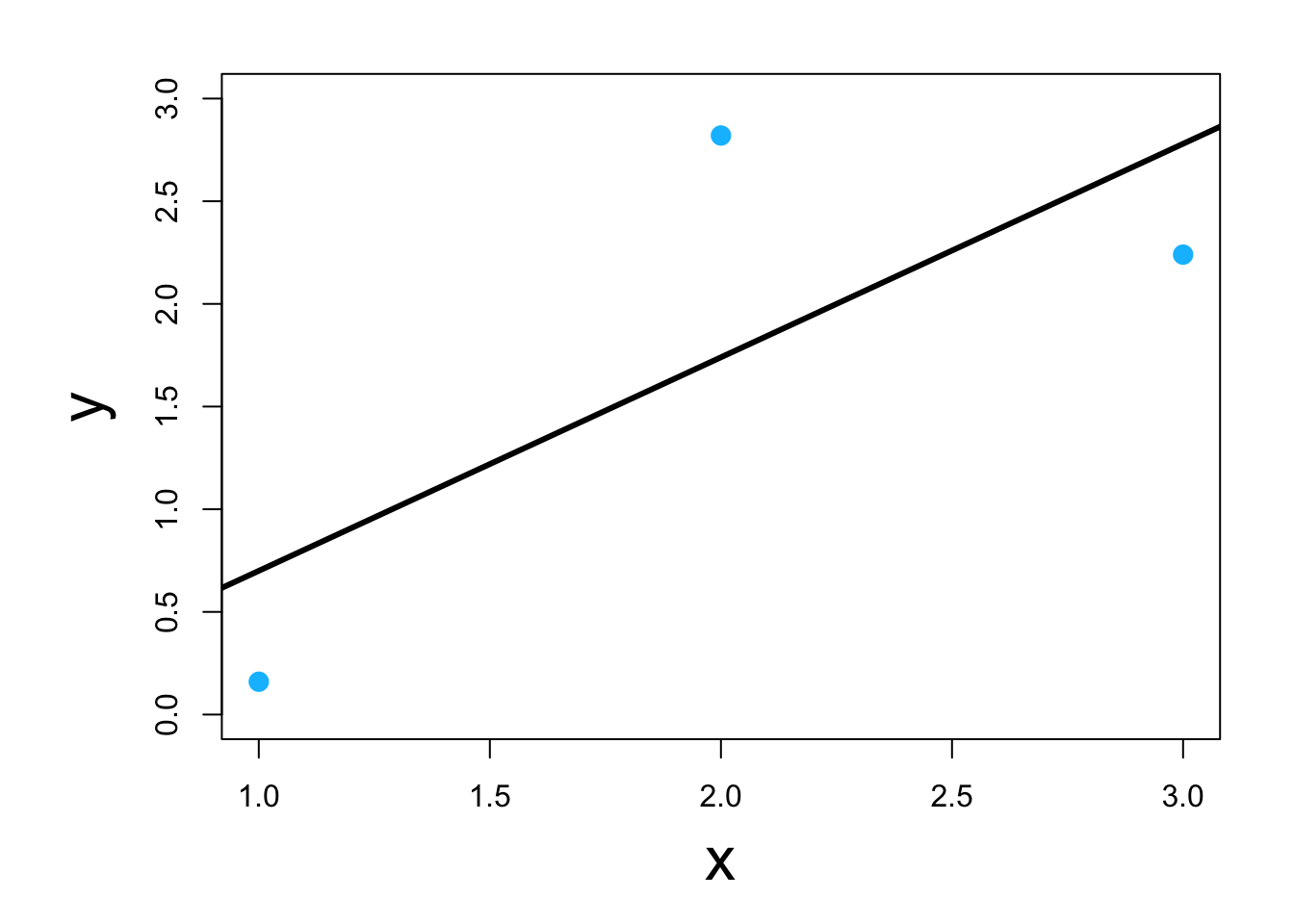
• Classic example $$\underset{\boldsymbol{\beta}}{\operatorname{argmin}}\sum_{i=1}^{n}(y_i-\mathbf{x}_{i}^{\prime}\boldsymbol{\beta})^2$$ or in matrix form $$\underset{\boldsymbol{\beta}}{\operatorname{argmin}}(\mathbf{y} - \mathbf{X}\boldsymbol{\beta})^{\prime}(\mathbf{y} - \mathbf{X}\boldsymbol{\beta})$$ which results in $$\hat{\boldsymbol{\beta}}=(\mathbf{X}^{\prime}\mathbf{X})^{-1}\mathbf{X}^{\prime}\mathbf{y}$$ -In R

  y <- c(0.16,2.82,2.24)
  X <- matrix(c(1,1,1,1,2,3),nrow=3,ncol=2,byrow=FALSE)
  
  solve(t(X)%*%X)%*%t(X)%*%y

  ##       [,1]
  ## [1,] -0.34
  ## [2,]  1.04

  optim(par=c(0,0),method = c("Nelder-Mead"),fn=function(beta){t(y-X%*%beta)%*%(y-X%*%beta)})

  ## $par
  ## [1] -0.3399977  1.0399687
  ## 
  ## $value
  ## [1] 1.7496
  ## 
  ## $counts
  ## function gradient 
  ##       61       NA 
  ## 
  ## $convergence
  ## [1] 0
  ## 
  ## $message
  ## NULL

  lm(y~X-1)

  ## 
  ## Call:
  ## lm(formula = y ~ X - 1)
  ## 
  ## Coefficients:
  ##    X1     X2  
  ## -0.34   1.04