37 Day 36 (July 27)
37.2 Regression trees
- Example: Change point analysis
- Motivation: Annual mean temperature in Ann Arbor Michigan
library(faraway)
plot(aatemp$year,aatemp$temp,xlab="Year",ylab="Annual mean temperature",pch=20,col=rgb(0.5,0.5,0.5,0.7))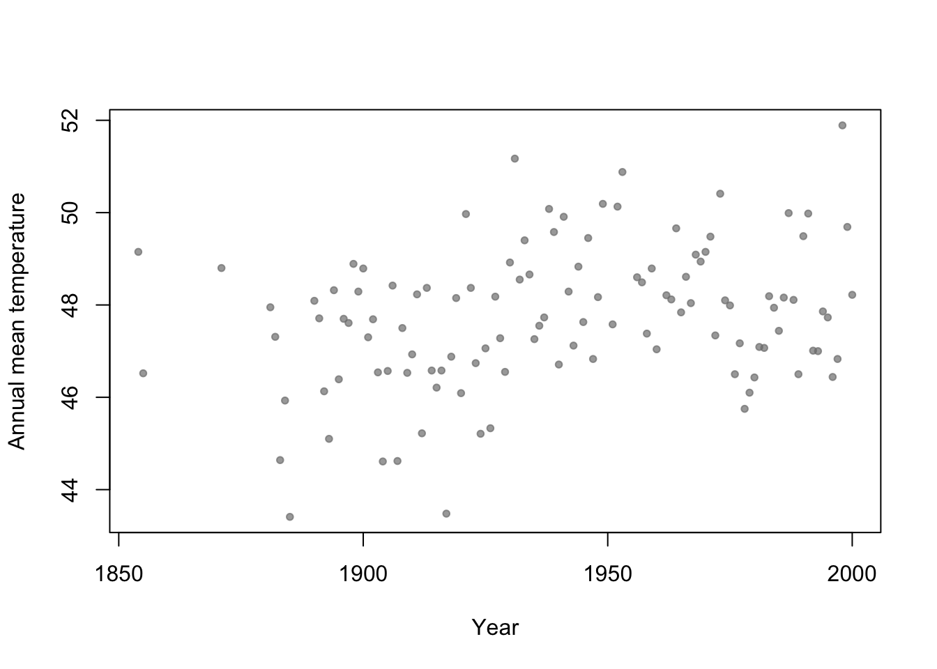
- Basis function \[f_1(x)=\begin{cases} 1 & \text{if}\;x<c\\ 0 & \text{otherwise} \end{cases}\] and \[f_2(x)=\begin{cases} 1 & \text{if}\;x\geq c\\ 0 & \text{otherwise} \end{cases}\]
- In R
# Change point basis function
f1 <- function(x,c){ifelse(x<c,1,0)}
f2 <- function(x,c){ifelse(x>=c,1,0)}

# Fit linear model
m1 <- lm(temp ~ -1 + f1(year,1930) + f2(year,1930),data=aatemp)
summary(m1)
## ## Call: ## lm(formula = temp ~ -1 + f1(year, 1930) + f2(year, 1930), data = aatemp) ## ## Residuals: ## Min 1Q Median 3Q Max ## -3.5467 -0.8962 -0.1157 1.1388 3.5843 ## ## Coefficients: ## Estimate Std. Error t value Pr(>|t|) ## f1(year, 1930) 46.9567 0.1990 236.0 <2e-16 *** ## f2(year, 1930) 48.3057 0.1684 286.8 <2e-16 *** ## --- ## Signif. codes: 0 '***' 0.001 '**' 0.01 '*' 0.05 '.' 0.1 ' ' 1 ## ## Residual standard error: 1.378 on 113 degrees of freedom ## Multiple R-squared: 0.9992, Adjusted R-squared: 0.9992 ## F-statistic: 6.899e+04 on 2 and 113 DF, p-value: < 2.2e-16# Plot predictions plot(aatemp$year,aatemp$temp,xlab="Year",ylab="Annual mean temperature",pch=20,col=rgb(0.5,0.5,0.5,0.7)) points(aatemp$year,predict(m1),type="l")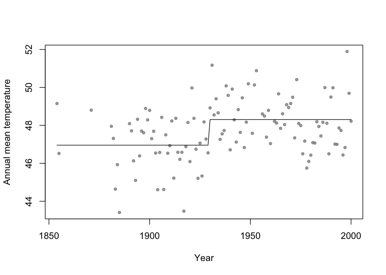
- Connection to regression trees
- For a single predictor, a regression tree can be though of as a linear model that uses the “change point” basis function, but tries to estimate the location (or time) and number of change points.
- Example in R
library(rpart)

# Fit regression tree model
m2 <- rpart(temp ~ year,data=aatemp)

# Plot predictions
E.y <- predict(m2,data.frame(year=seq(1850,2023,by=1)))
plot(aatemp$year,aatemp$temp,xlab="Year",ylab="Annual mean temperature",pch=20,col=rgb(0.5,0.5,0.5,0.7),xlim=c(1850,2023))
points(1850:2023,E.y,type="l")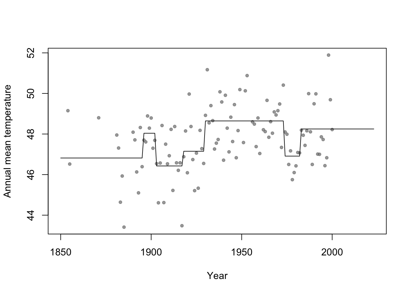
37.3 Random forest
Breiman 2001 link
Example
n.boot <- 1000 # Number of bootstrap samples
x.new=seq(1850,2023,by=1) # New values of x that I want predicitons at
E.y <- matrix(,length(x.new),n.boot) # Matrix to save predictions
x <- aatemp$year
y <- aatemp$temp

for(i in 1:n.boot){

  # Resample data
  df.temp <- data.frame(y=y,x=x)[sample(1:length(y),replace=TRUE,size=51),]

  # Fit tree
  m1 <- rpart(y~x,data=df.temp)

  # Get and save predictions
  E.y[,i] <- predict(m1,data.frame(x=x.new))
}

plot(aatemp$year,aatemp$temp,xlab="Year",ylab="Annual mean temperature",pch=20,col=rgb(0.5,0.5,0.5,0.7),xlim=c(1850,2023))


# Aggregate predictions
E.E.y <- rowMeans(E.y)
points(1850:2023,E.E.y,type="l")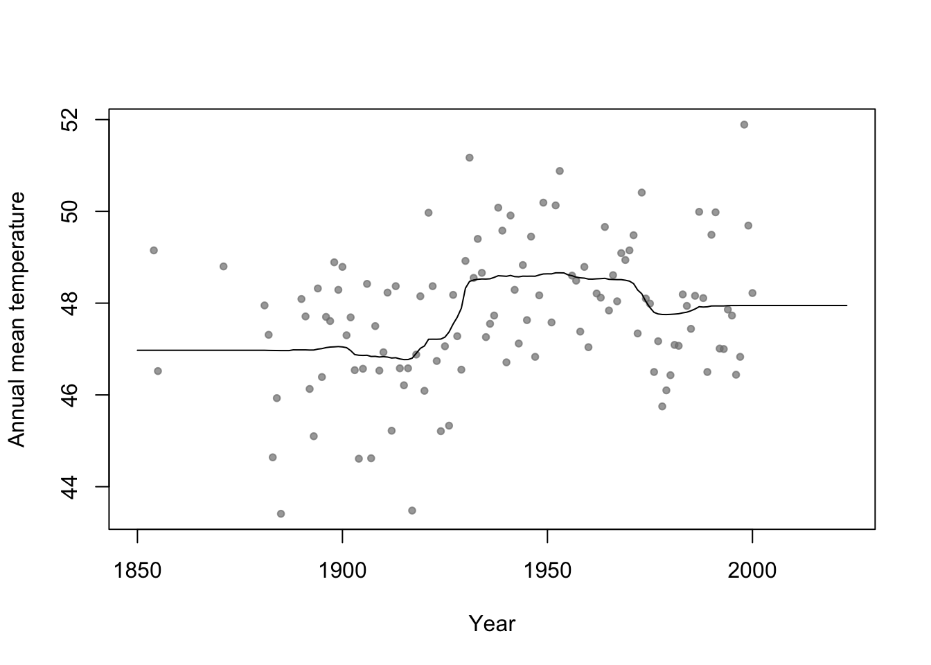
Summary
- Bootstrap aggregating (or bagging) can be used with any statistical model
- Usually increases predictive accuracy but reduces ability to understand (and write-out) the model(s) and make inference
37.4 Generalized additive model
- Write out on white board
- Difference between interpretable vs. non-interpretable model/machine learning approaches
- My personal use of gams
- The functions lm() and glm() and packages lme4, nlme, etc
- Why I use the mgcv package
- Wood (2017)
- The functions lm() and glm() and packages lme4, nlme, etc
- Example
library(faraway)
library(mgcv)
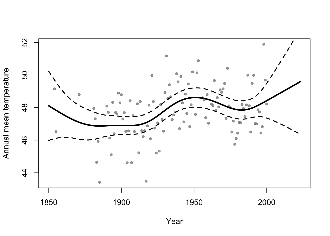
m1 <- gam(temp ~ s(year,bs="tp"),family=Gamma(link="log"),data=aatemp)
# Plot predictions
E.y <- predict(m1,data.frame(year=seq(1850,2023,by=1)),type="response")
ui <- E.y + 1.96*predict(m1,data.frame(year=seq(1850,2023,by=1)),type="response",se=TRUE)$se.fit
li <- E.y - 1.96*predict(m1,data.frame(year=seq(1850,2023,by=1)),type="response",se=TRUE)$se.fit
plot(aatemp$year,aatemp$temp,xlab="Year",ylab="Annual mean temperature",pch=20,col=rgb(0.5,0.5,0.5,0.7),xlim=c(1850,2023))
points(1850:2023,E.y,type="l",lwd=3)
points(1850:2023,ui,type="l",lwd=2,lty=2)
points(1850:2023,li,type="l",lwd=2,lty=2)