16 Day 16 (June 26)
16.2 Bootstrap confidence intervals
- Finish up notes from Friday (mosaic package, other other derived quantities)
- Live example
16.3 Prediction
- My definition of inference and prediction
- Inference = Learning about what you can’t observe given what you did observe (and some assumptions)
- Prediction = Learning about what you didn’t observe given what you did observe (and some assumptions)
- Prediction (Ch. 4 in Faraway (2014))
- Derived quantity
- \(\mathbf{x}^{\prime}_0\) is a \(1\times p\) matrix of covariates (could be a row \(\mathbf{X}\) or completely new values of the predictors)
- Use \(\widehat{\text{E}(y_0)}=\mathbf{x}^{\prime}_0\hat{\boldsymbol{\beta}}\)
- Example
- Predicting the number of whooping cranes
url <- "https://www.dropbox.com/s/8grip274233dr9a/Butler%20et%20al.%20Table%201.csv?dl=1"
df1 <- read.csv(url)

plot(df1$Winter, df1$N, xlab = "Year", ylab = "Population size",
xlim=c(1940,2021),ylim = c(0, 300), typ = "b", lwd = 1.5, pch = "*")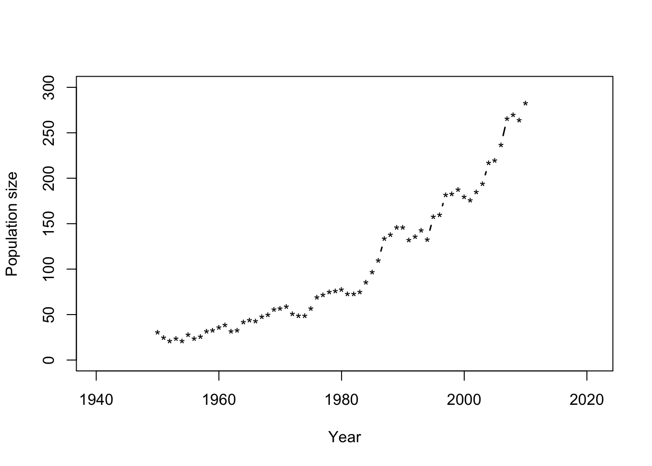
- What model should we use?
m1 <- lm(N ~ Winter + I(Winter^2),data=df1)
Ey.hat <- predict(m1)

plot(df1$Winter, df1$N, xlab = "Year", ylab = "Population size",
xlim=c(1940,2021),ylim = c(0, 300), typ = "b", lwd = 1.5, pch = "*")
points(df1$Winter,Ey.hat,typ="l",col="red")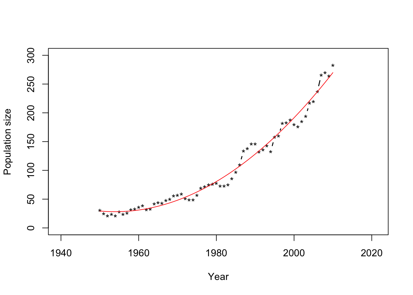
- Derived quantity
16.4 Intervals for predictions
- Expected value and variance of \(\mathbf{x}^{\prime}_0\hat{\boldsymbol{\beta}}\)
- Confidence interval \(\text{P}\left(\mathbf{x}^{\prime}_0\hat{\boldsymbol{\beta}}-t_{\alpha/2,n-p}\sqrt{\hat{\sigma^{2}}\mathbf{x}_{0}^{'}(\mathbf{X}^{'}\mathbf{X})^{-1}\mathbf{x}_{0}}<\mathbf{x}^{\prime}_0\boldsymbol{\beta}<\mathbf{x}^{\prime}_0\hat{\boldsymbol{\beta}}+t_{\alpha/2,n-p}\sqrt{\hat{\sigma^{2}}\mathbf{x}_{0}^{'}(\mathbf{X}^{'}\mathbf{X})^{-1}\mathbf{x}_{0}}\right)\\=1-\alpha\)
- The 95% CI is \(\mathbf{x}^{\prime}_0\hat{\boldsymbol{\beta}}\pm t_{\alpha/2,n-p}\sqrt{\hat{\sigma^{2}}\mathbf{x}_{0}^{'}(\mathbf{X}^{'}\mathbf{X})^{-1}\mathbf{x}_{0}}\)
- In R
Ey.hat <- predict(m1,interval="confidence")
head(Ey.hat)
## fit lwr upr ## 1 29.35980 21.43774 37.28186 ## 2 28.84122 21.42928 36.25315 ## 3 28.47610 21.54645 35.40575 ## 4 28.26444 21.78812 34.74075 ## 5 28.20624 22.15308 34.25940 ## 6 28.30150 22.64000 33.96300plot(df1$Winter, df1$N, xlab = "Year", ylab = "Population size", xlim=c(1940,2021),ylim = c(0, 300), typ = "b", lwd = 1.5, pch = "*") points(df1$Winter,Ey.hat[,1],typ="l",col="red") points(df1$Winter,Ey.hat[,2],typ="l",col="red",lty=2) points(df1$Winter,Ey.hat[,3],typ="l",col="red",lty=2)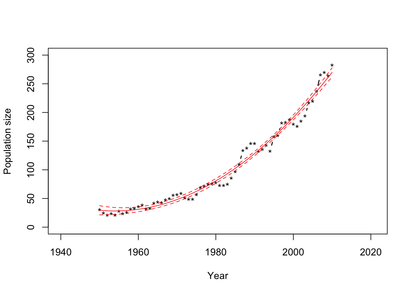
- Why are there so many data points that fall outside of the 95% CIs?
- Prediction intervals vs. Confidence intervals
CIs for \(\widehat{\text{E}(y_0)}=\mathbf{x}^{\prime}_0\hat{\boldsymbol{\beta}}\)
How to interpret \(\widehat{\text{E}(y_0)}\)
What if I wanted to predict \(y_0\)?
- \(y_0\sim\text{N}(\mathbf{x}^{\prime}_0\hat{\boldsymbol{\beta}},\hat{\sigma}^2)\)
Expected value and variance of \(y_0\)
Prediction interval \(\text{P}\left(\mathbf{x}^{\prime}_0\hat{\boldsymbol{\beta}}-t_{\alpha/2,n-p}\sqrt{\hat{\sigma^{2}}(1+\mathbf{x}_{0}^{'}(\mathbf{X}^{'}\mathbf{X})^{-1}\mathbf{x}_{0})}<y_0<\mathbf{x}^{\prime}_0\hat{\boldsymbol{\beta}}+t_{\alpha/2,n-p}\sqrt{\hat{\sigma^{2}}(\mathbf{x}_{0}^{'}(\mathbf{X}^{'}\mathbf{X})^{-1}\mathbf{x}_{0})}\right)=\\1-\alpha\)
The 95% PI is \(\mathbf{x}^{\prime}_0\hat{\boldsymbol{\beta}}\pm t_{\alpha/2,n-p}\sqrt{\hat{\sigma^{2}}(1+\mathbf{x}_{0}^{'}(\mathbf{X}^{'}\mathbf{X})^{-1}\mathbf{x}_{0})}\)
Example in R
y.hat <- predict(m1,interval="prediction")
head(y.hat)
## fit lwr upr
## 1 29.35980 6.630220 52.08938
## 2 28.84122 6.284368 51.39807
## 3 28.47610 6.073089 50.87910
## 4 28.26444 5.997480 50.53139
## 5 28.20624 6.058655 50.35382
## 6 28.30150 6.257741 50.34526plot(df1$Winter, df1$N, xlab = "Year", ylab = "Population size",
xlim=c(1940,2021),ylim = c(0, 300), typ = "b", lwd = 1.5, pch = "*")
points(df1$Winter,y.hat[,1],typ="l",col="red")
points(df1$Winter,y.hat[,2],typ="l",col="red",lty=2)
points(df1$Winter,y.hat[,3],typ="l",col="red",lty=2)
References
Faraway, J. J. 2014. Linear Models with r. CRC Press.