15 Day 15 (June 23)

15.1 Announcements

Read Ch. 4 in linear models with R

15.2 Confidence intervals for derived quantities

Delta method live example

15.3 Bootstrap confidence intervals

Google scholar demonstration

Motivation (see section 3.6 in Faraway (2014))

Functions of parameters (i.e., “derived” quantities)
Difficult to obtain the sampling distribution for non-linear functions of estimated parameters
Further reading (Hesterberg 2015)
Example: When do we expect the population to go extinct?

y <- c(63, 68, 61, 44, 103, 90, 107, 105, 76, 46, 60, 66, 58, 39, 64, 29, 37,
27, 38, 14, 38, 52, 84, 112, 112, 97, 131, 168, 70, 91, 52, 33, 33, 27,
18, 14, 5, 22, 31, 23, 14, 18, 23, 27, 44, 18, 19)
year <- 1965:2011
df <- data.frame(y = y, year = year)
plot(x = df$year, y = df$y, xlab = "Year", ylab = "Annual count", main = "",
col = "brown", pch = 20, xlim = c(1965, 2040))
m1 <- lm(y~year)
abline(m1)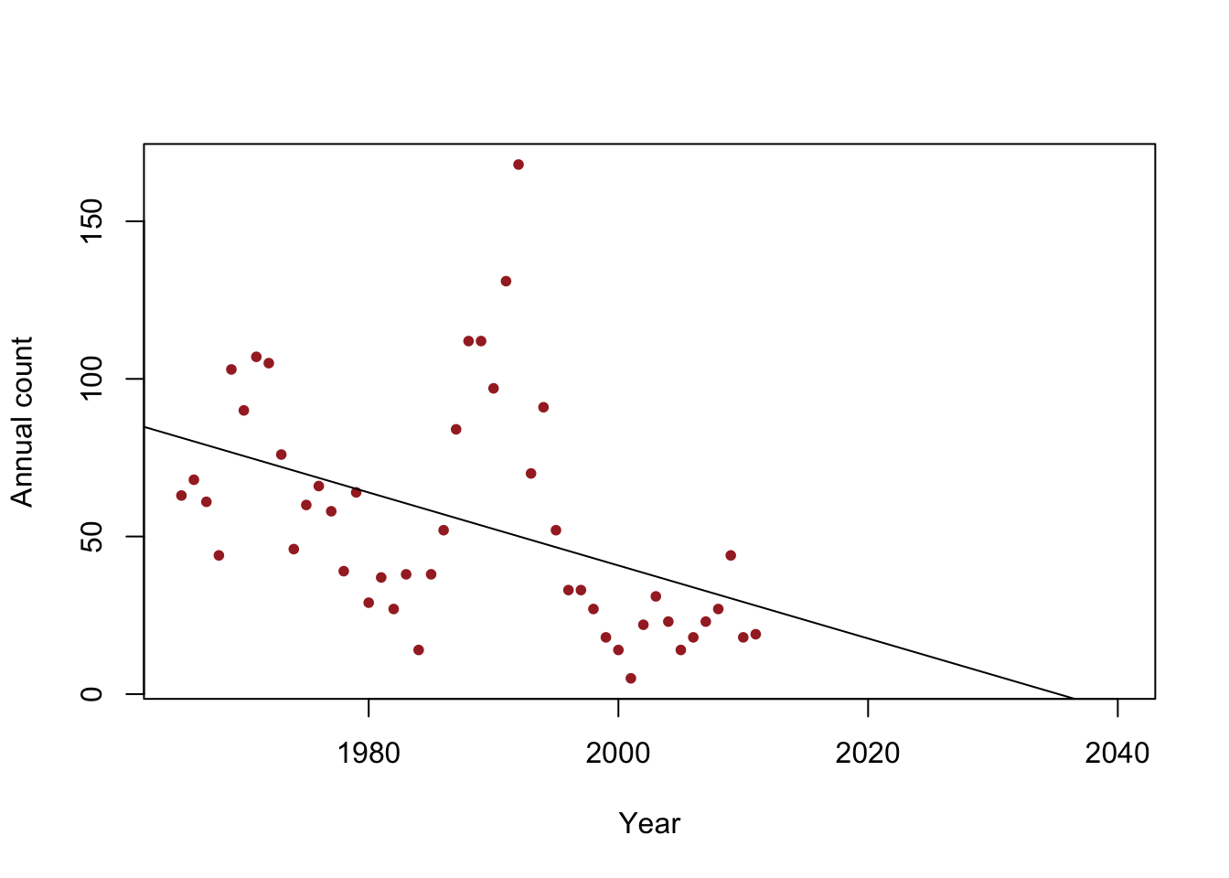

Non-parametric bootstrap (see Efron and Tibshirani (1994)).
1. From a data set with n observations, take a sample of size n with replacement. For a linear model, the sample should include both the observed response (\(y_{i}\)) and covariates (\(x_{1}\),\(x_{2}\),…,\(x_{p}\)).
2. Estimate the parameters for a statistical model using the sampled data from step 1.
3. Save the estimates of interest. This could be parameters of interest (e.g., \(\boldsymbol{\beta}\)) or a a derived quantity (e.g., \(R^{2}\), \(\frac{1}{\boldsymbol{\beta}}\)).
4. Repeats steps (1)-(3) \(m\) times.
Inference
- The \(m\) samples of the quantities of interest are samples from the empirical distribution.
- The empirical distribution can summarized using sample statistics (e.g., quantiles, mean, variance, etc). Conceptually, this is similar to Monte Carlo integration.

Example in R

library(latex2exp)
# Number of bootstrap samples (m)
m.boot <- 1000   

# Create matrix to save empirical distribution of -beta2.hat/beta1.hat (expected time of extinction)
ed.extinct.hat <- matrix(,m.boot,1)

# Set random seed so results are the same if we run it again
# Results would be different due to random resampling of data
set.seed(1940)   

# Start for loop for non-parametric boostrap
for(m in 1:m.boot){

  # Sample data with replacement
  # boot.sample gives the rows of df that we use for estimation
  boot.sample <- sample(1:nrow(df),replace=TRUE) 

  # Make temporary data frame that contains the resamples
  df.temp <- df[boot.sample,]

  # Estimate parameters for df.temp
  m1 <- lm(y~year,data=df.temp)

  # Save estimate of -beta0.hat/beta1.hat (expected time of extinction)
  ed.extinct.hat[m,] <- -coef(m1)[1]/coef(m1)[2]
}
par(mar=c(5,4,7,2))
hist(ed.extinct.hat,col="grey",xlab="Year",main=TeX('Empirical distribuiton of $$-$$\\hat{\\frac{$\\beta_0}{$\\beta_1}}'),freq=FALSE,breaks=20)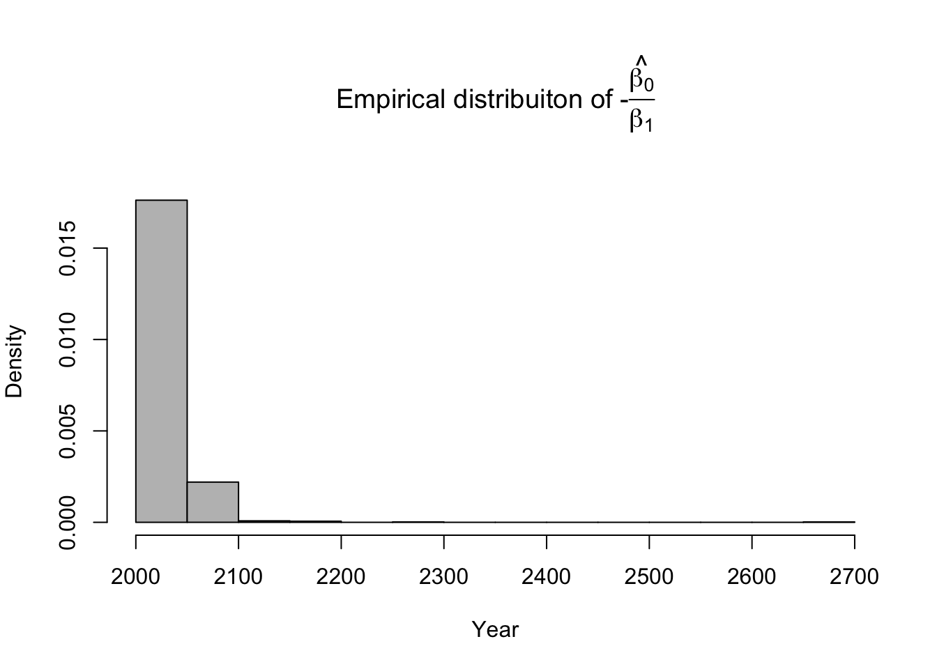

# 95% equal-tailed CI based on percentiles of the empirical distribution
quantile(ed.extinct.hat,prob=c(0.025,0.975))

##     2.5%    97.5% 
## 2021.203 2077.168

Example in R using the mosaic package

library(mosaic)

set.seed(1940) 
bootstrap <- do(1000)*coef(lm(y~year,data=resample(df)))
head(bootstrap)

##   Intercept       year
## 1  1703.401 -0.8291862
## 2  3017.102 -1.4887107
## 3  2683.814 -1.3195092
## 4  2595.994 -1.2778627
## 5  2334.905 -1.1463994
## 6  2011.819 -0.9811046

# 95% equal-tailed CI based on percentiles of the empirical distribution
quantile(-bootstrap[,1]/bootstrap[,2],prob=c(0.025,0.975))

##     2.5%    97.5% 
## 2021.203 2077.168

confint(bootstrap,method="percentile") # Comparison of 95% CI with traditional approach

##   name     lower      upper level     method estimate
## 1 year -1.623489 -0.6753815  0.95 percentile -1.15784

confint(m1)[2,]

##      2.5 %     97.5 % 
## -1.9107236 -0.5405716

Live example

References

Efron, Bradley, and Robert J Tibshirani. 1994. An Introduction to the Bootstrap. CRC press.

Faraway, J. J. 2014. Linear Models with r. CRC Press.

Hesterberg, Tim C. 2015. “What Teachers Should Know about the Bootstrap: Resampling in the Undergraduate Statistics Curriculum.” The American Statistician 69 (4): 371–86.