1.4 Transformations of random vectors

The following result allows obtaining the distribution of a random vector $\boldsymbol{Y}=g(\boldsymbol{X})$ from that of $\boldsymbol{X},$ if $g$ is a sufficiently well-behaved function.

Theorem 1.4 (Injective transformation of continuous random vectors) Let $\boldsymbol{X}\sim f_{\boldsymbol{X}}$ be a continuous random vector in $\mathbb{R}^p.$ Let $g=(g_1,\ldots,g_p):\mathbb{R}^p\rightarrow\mathbb{R}^p$ be such that:²⁰

$g$ is injective;²¹
the partial derivatives $\frac{\partial g_i}{\partial x_j} :\mathbb{R}^p\rightarrow\mathbb{R}$ exist and are continuous almost everywhere, for $i,j=1,\ldots,p;$
for almost all $\boldsymbol{y}\in\mathbb{R}^p,$ $\left\|\frac{\partial g^{-1}(\boldsymbol{y})}{\partial \boldsymbol{y}}\right\|\neq0.$²²

Then, $\boldsymbol{Y}=g(\boldsymbol{X})$ is a continuous random vector in $\mathbb{R}^p$ whose pdf is

\[\begin{align*} f_{\boldsymbol{Y}}(\boldsymbol{y})=f_{\boldsymbol{X}}\big(g^{-1}(\boldsymbol{y})\big) \left\|\frac{\partial g^{-1}(\boldsymbol{y})}{\partial \boldsymbol{y}}\right\|,\quad \boldsymbol{y}\in\mathbb{R}^p. \end{align*}\]

Example 1.32 Consider the random vector $(X,Y)'$ with pdf

\[\begin{align*} f_{(X,Y)}(x,y)=\begin{cases} 2/9,&0<x<3,\ 0<y<x<3, \\ 0,&\text{otherwise.} \end{cases} \end{align*}\]

What are the distributions of $X+Y$ and $X-Y$?

To answer this question, we define

\[\begin{align*} g(x,y)=(x+y,x-y)'=(u,v)' \end{align*}\]

and seek to apply Theorem 1.4. Since $g^{-1}(u,v)=((u+v)/2,(u-v)/2)',$ then

\[\begin{align*} \left\|\frac{\partial g^{-1}(\boldsymbol{y})}{\partial \boldsymbol{y}}\right\|=\left\|\begin{pmatrix} 1/2&1/2\\ 1/2&-1/2\\ \end{pmatrix}\right\|=\left|-\frac{1}{4}-\frac{1}{4}\right|=\frac{1}{2}\neq0. \end{align*}\]

Then, Theorem 1.4 is applicable and $(U,V)'=g(X,Y)$ has pdf

\[\begin{align*} f_{(U,V)}(u,v)&=f_{(X,Y)}\big(g^{-1}(u,v)\big)\frac{1}{2}\\ &=\begin{cases} 1/9,&0<(u+v)/2<3,\ 0<(u-v)/2<(u+v)/2<3,\\ 0,&\text{otherwise.} \end{cases} \end{align*}\]

Observe that $V>0$ by definition. Hence, we can rewrite $f_{(U,V)}(u,v)=\frac{1}{9}1_{\{(u,v)'\in S\}},$ where the support $S=\{(u,v)'\in\mathbb{R}^2:0<v<6-u,\ 0<v<u\}$ is a triangular region delimited by $v=0,$ $u=v,$ and $u+v=6$ (a triangle with vertexes on $(0,0),$ $(3,3),$ and $(6,0)$ — draw it for graphical insight!).

This insight is important to compute the marginals of $(U,V),$ which give the distributions of $X+Y$ and $X-Y$:

\[\begin{align*} f_{U}(u)&=\int_{\mathbb{R}} \frac{1}{9}1_{\{(u,v)'\in S\}}\,\mathrm{d}v=\begin{cases} \int_{0}^{u}1/9\,\mathrm{d}v=u/9,& u\in(0,3),\\ \int_{0}^{6-u}1/9\,\mathrm{d}v=(6-u)/9,&u\in(3,6),\\ 0,&\text{otherwise,} \end{cases}\\ f_{V}(v)&=\int_{\mathbb{R}} \frac{1}{9}1_{\{(u,v)'\in S\}}\,\mathrm{d}u=\begin{cases} \int_{v}^{6-v}1/9\,\mathrm{d}u=(6-2v)/9,& v\in(0,3),\\ 0,&\text{otherwise.} \end{cases} \end{align*}\]

Remark. If the function $g$ is only injective over the support of $\boldsymbol{X},$ Theorem 1.4 still can be applied. For example, $g(x)=\sin(x)$ is (in particular) injective in $(-\pi/2,\pi/2),$ but is not injective in $\mathbb{R}.$ Following with the example, the pdf of $Y=\sin(X)$ if $X\sim \mathcal{U}(0,\pi/2)$ is

\[\begin{align*} f_Y(y)=\frac{2}{\pi} \left|\frac{\mathrm{d}}{\mathrm{d} y}\arcsin(y)\right| 1_{\left\{\arcsin(y)\in \left(0,\tfrac{\pi}{2}\right)\right\}}=\frac{2}{\pi\sqrt{1-y^2}} 1_{\{y\in (0,1)\}}. \end{align*}\]

What if we wanted to know the distribution of the random variable $Z=g_1(\boldsymbol{X})$ from that of the random vector $\boldsymbol{X}\sim f_{\boldsymbol{X}}$? The trick done in the example above points towards the approach to solve this case. Since $g_1:\mathbb{R}^p\rightarrow\mathbb{R},$ we cannot directly apply Theorem 1.4. However, what we can do is:

Complement $g_1$ to $g:\mathbb{R}^p\rightarrow\mathbb{R}^p$ so that $g$ satisfies Theorem 1.4. For example, by defining $g(\boldsymbol{x})=(g_1(\boldsymbol{x}),x_2,\ldots,x_p)$ (this heavily depends on the form of $g_1$).
Marginalize $\boldsymbol{Y}=g(\boldsymbol{X})$ to get the first marginal pdf, i.e., the pdf of $Z.$

The next corollary works out the application of the previous principle for sums of independent random variables.

Corollary 1.2 (Sum of independent and continuous random variables) Let $X_i\sim f_{X_i},$ $i=1,\ldots,n,$ be independent and continuous random variables. The pdf of $S:=X_1+\cdots+X_n$ is

\[\begin{align} f_S(s)=\int_{\mathbb{R}^{n-1}} f_{X_1}(s-x_2-\cdots-x_{n}) f_{X_2}(x_2)\cdots f_{X_n}(x_n) \,\mathrm{d} x_2\cdots\,\mathrm{d} x_n. \tag{1.10} \end{align}\]

Proof (Proof of Corollary 1.2). The pdf of $S$ can be obtained using the transformation

\[\begin{align*} g\begin{pmatrix}x_1\\x_2\\\vdots\\x_n\end{pmatrix}=\begin{pmatrix}x_1+\cdots+x_n\\x_2\\\vdots\\x_n\end{pmatrix},\quad g^{-1}\begin{pmatrix}y_1\\y_2\\\vdots\\y_n\end{pmatrix}=\begin{pmatrix}y_1-y_2-\cdots-y_n\\y_2\\\vdots\\y_n\end{pmatrix} \end{align*}\]

with

\[\begin{align*} \left\|\frac{\partial g^{-1}(\boldsymbol y)}{\partial \boldsymbol y}\right\|=\left\|\begin{pmatrix} 1 & -1 & \cdots & -1\\ 0 & 1 & \cdots & 0 \\ \vdots & \vdots & \ddots & \vdots \\ 0 & 0 & \cdots & 1 \\ \end{pmatrix}\right\|=1 \end{align*}\]

Because of Theorem 1.4 and independence, the pdf of $\boldsymbol{Y}=g(\boldsymbol{X})$ is

\[\begin{align*} f_{\boldsymbol{Y}}(\boldsymbol{y})&=f_{\boldsymbol{X}}(y_1-y_2-\cdots-y_n,y_2,\ldots,y_n)\\ &=f_{X_1}(y_1-y_2-\cdots-y_n)f_{X_2}(y_2)\cdots f_{X_n}(y_n). \end{align*}\]

A posterior marginalization for $Y_1=S$ gives

\[\begin{align*} f_{Y_1}(y_1)=\int_{\mathbb{R}^{n-1}} f_{X_1}(y_1-y_2-\cdots-y_n)f_{X_2}(y_2)\cdots f_{X_n}(y_n)\, \mathrm{d}y_2\cdots\, \mathrm{d}y_n. \end{align*}\]

Remark. Care is needed on the domain of integration of (1.10), which is implicitly informed by the domains of $f_{X_1}$ and $f_{X_2}.$

There are more cumbersome or challenging situations involving transformations of random vectors than those covered by Theorem 1.4. For example, those dealing with a transformation $g$ that is non-injective over the support of $\boldsymbol{X}.$ In that case, roughly speaking, one needs to break the support of $\boldsymbol{X}$ into “injective pieces” $\Delta_1,\Delta_2,\ldots$ for which $g$ is injective, apply Theorem 1.4 in each of the pieces, and then combine adequately the resulting pdfs.

Theorem 1.5 (Non-injective transformation of continuous random vectors) Let $\boldsymbol{X}\sim f_{\boldsymbol{X}}$ be a continuous random vector in $\mathbb{R}^p.$ Let $g:\mathbb{R}^p\rightarrow\mathbb{R}^p$ be such that:

There exists a partition $\Delta_1,\Delta_2,\ldots$ of $\mathbb{R}^p$ where the restrictions of $g$ to each $\Delta_i,$ denoted by $g_{\Delta_i},$ are injective.
All the functions $g_{\Delta_i}:\mathbb{R}^p\rightarrow\mathbb{R}^p$ verify the assumptions ii and iii of Theorem 1.4.

Then $\boldsymbol{Y}=g(\boldsymbol{X})$ is a continuous random vector in $\mathbb{R}^p$ whose pdf is

\[\begin{align} f_{\boldsymbol{Y}}(\boldsymbol{y})=\sum_{\{i :\ \boldsymbol{y}\in g_{\Delta_i}(\Delta_i)\}} f_{\boldsymbol{X}}\big(g_{\Delta_i}^{-1}(\boldsymbol{y})\big) \left\|\frac{\partial g_{\Delta_i}^{-1}(\boldsymbol{y})}{\partial \boldsymbol{y}}\right\|,\quad \boldsymbol{y}\in\mathbb{R}^p.\tag{1.11} \end{align}\]

$Non-injective function $g.$$

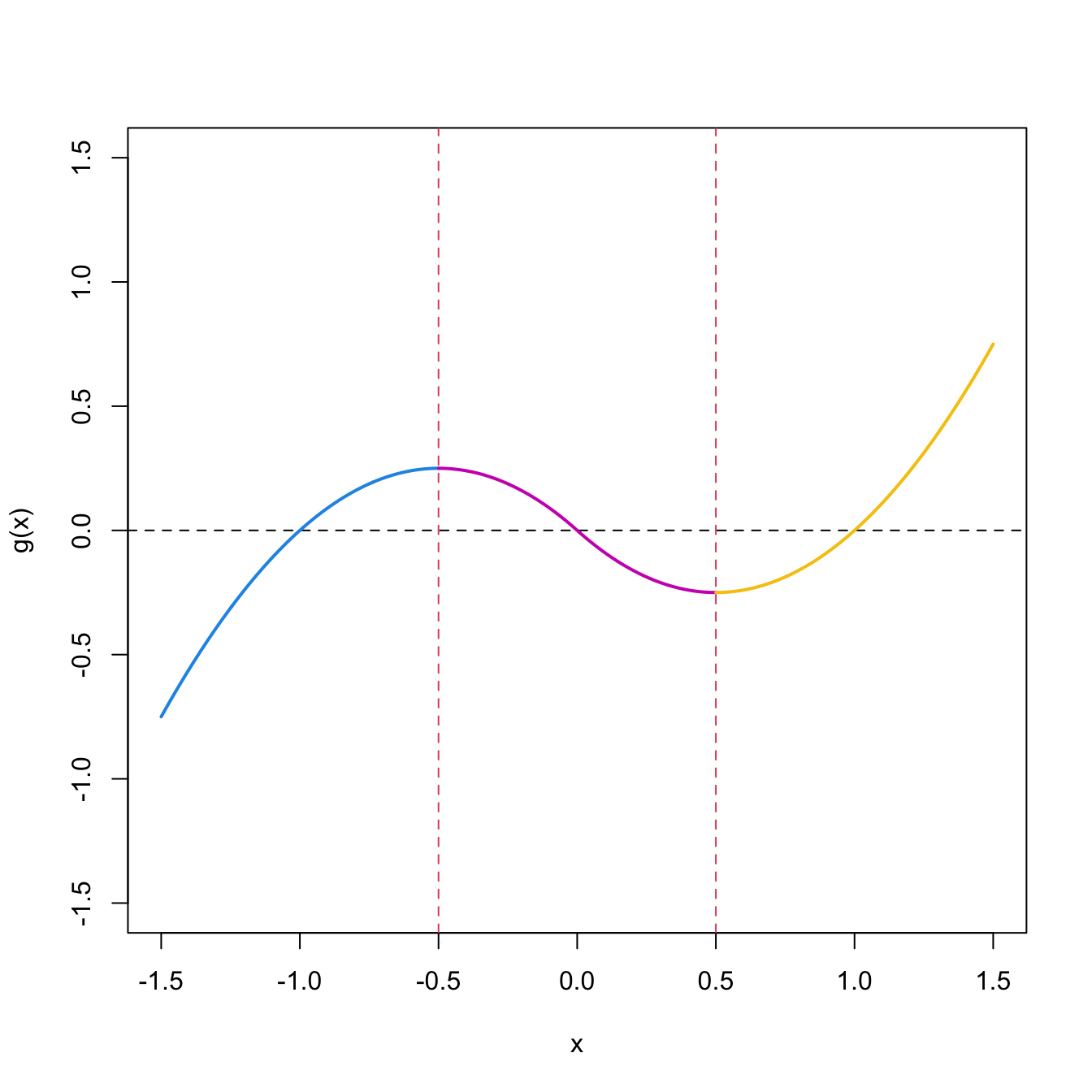
Figure 1.11: Non-injective function $g.$

$Injective partition $\Delta_i,$ $i=1,2,3,$ and injective restrictions $g_{\Delta_i}.$$

Figure 1.12: Injective partition $\Delta_i,$ $i=1,2,3,$ and injective restrictions $g_{\Delta_i}.$

$Limits of $g_{\Delta_i}(\Delta_i),$ $i=1,2,3.$$

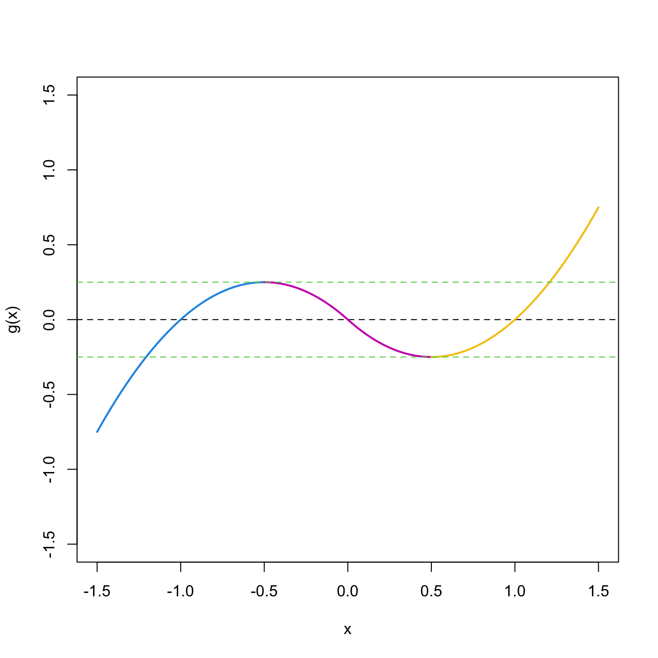
Figure 1.13: Limits of $g_{\Delta_i}(\Delta_i),$ $i=1,2,3.$

Example 1.33 Consider $g(x)=-x(x+1)1_{\{x<0\}}+x(x-1)1_{\{x>0\}}.$ This is a very smooth function, but is non-injective (e.g., $-1,$ $0,$ and $1$ all map to zero, see Figure 1.11). We can see what are its relative extrema to determine the injective regions: $\frac{\mathrm{d} g(x)}{\mathrm{d} x}=-(2x+1)_{\{x<0\}}+(2x-1)1_{\{x>0\}}=0\iff x=\pm 1/2.$ This gives the following partition for which $g$ is piecewise injective (see Figure 1.12):²³

\[\begin{align*} \Delta_1=(-\infty, -1/2],\ \Delta_2=(-1/2, 1/2),\text{ and } \Delta_3=[1/2,\infty). \end{align*}\]

Now, for each $\Delta_i,$ we can invert $g_{\Delta_i}.$ For that, we keep in mind where $g_{\Delta_i}$ are mapping at, i.e., what are $g_{\Delta_i}(\Delta_i)$ (see Figure 1.13):

For $y\in g_{\Delta_1}(\Delta_1)=(-\infty,1/4],$ $g_{\Delta_1}^{-1}(y)=(-1-\sqrt{1-4y})/2$ from solving $y=-x^2-x.$ Then, $\frac{\mathrm{d} g_{\Delta_1}^{-1}(y)}{\mathrm{d} y}=(1-4y)^{-1/2}.$
For $y\in g_{\Delta_2}(\Delta_2)=(-1/4,1/4),$ \[\begin{align*} g_{\Delta_2}^{-1}(y)=\begin{cases} (1-\sqrt{1+4y})/2,& y\in(-1/4,0),\\ (-1+\sqrt{1-4y})/2,& y\in(0,1/4) \end{cases} \end{align*}\] from solving $y=-x^2-x$ and $y=x^2-x,$ respectively. Then, \[\begin{align*} \frac{\mathrm{d} g_{\Delta_2}^{-1}(y)}{\mathrm{d} y}=\begin{cases} -(1+4y)^{-1/2},& y\in(-1/4,0),\\ -(1-4y)^{-1/2},& y\in(0,1/4). \end{cases} \end{align*}\]
For $y\in g_{\Delta_3}(\Delta_3)=[-1/4,\infty),$ $g_{\Delta_3}^{-1}(y)=(1+\sqrt{1+4y})/2$ from solving $y=x^2-x.$ Then, $\frac{\mathrm{d} g_{\Delta_3}^{-1}(y)}{\mathrm{d} y}=(1+4y)^{-1/2}.$

Observe that $g_{\Delta_i}(\Delta_i),$ $i=1,2,3$ are overlapping! This is what (1.11) is implicitly warning us with its variable sum: when there is no overlapping, only one pdf is in the sum, but when there is, then several pdfs will enter the sum. We can now proceed applying (1.11) for any $f_X$:

\[\begin{align*} f_Y(y)=&\;\sum_{\{i :\ y\in g_{\Delta_i}(\Delta_i)\}} f_X\big(g_{\Delta_i}^{-1}(y)\big) \left|\frac{\mathrm{d} g_{\Delta_i}^{-1}(y)}{\mathrm{d} y}\right|\\ =&\;\begin{cases} f_X\big(g_{\Delta_1}^{-1}(y)\big) \left|\frac{\mathrm{d} g_{\Delta_1}^{-1}(y)}{\mathrm{d} y}\right| ,&y\in(-\infty,-1/4],\\ \sum_{i=1}^3 f_X\big(g_{\Delta_i}^{-1}(y)\big) \left|\frac{\mathrm{d} g_{\Delta_i}^{-1}(y)}{\mathrm{d} y}\right| ,&y\in(-1/4,1/4),\\ f_X\big(g_{\Delta_3}^{-1}(y)\big) \left|\frac{\mathrm{d} g_{\Delta_3}^{-1}(y)}{\mathrm{d} y}\right| ,&y\in[1/4,\infty). \end{cases} \end{align*}\]

Remark. The collection $\Delta_1,\Delta_2,\ldots$ that injectivizes $g$ might not be finite. For example, if $g(x)=\sin(x),$ then such collection is $\{\Delta_k\}_{k\in\mathbb{Z}}$ with $\Delta_k=(-\pi/2+k\pi,\pi/2+k\pi)$ (Figure 1.14).

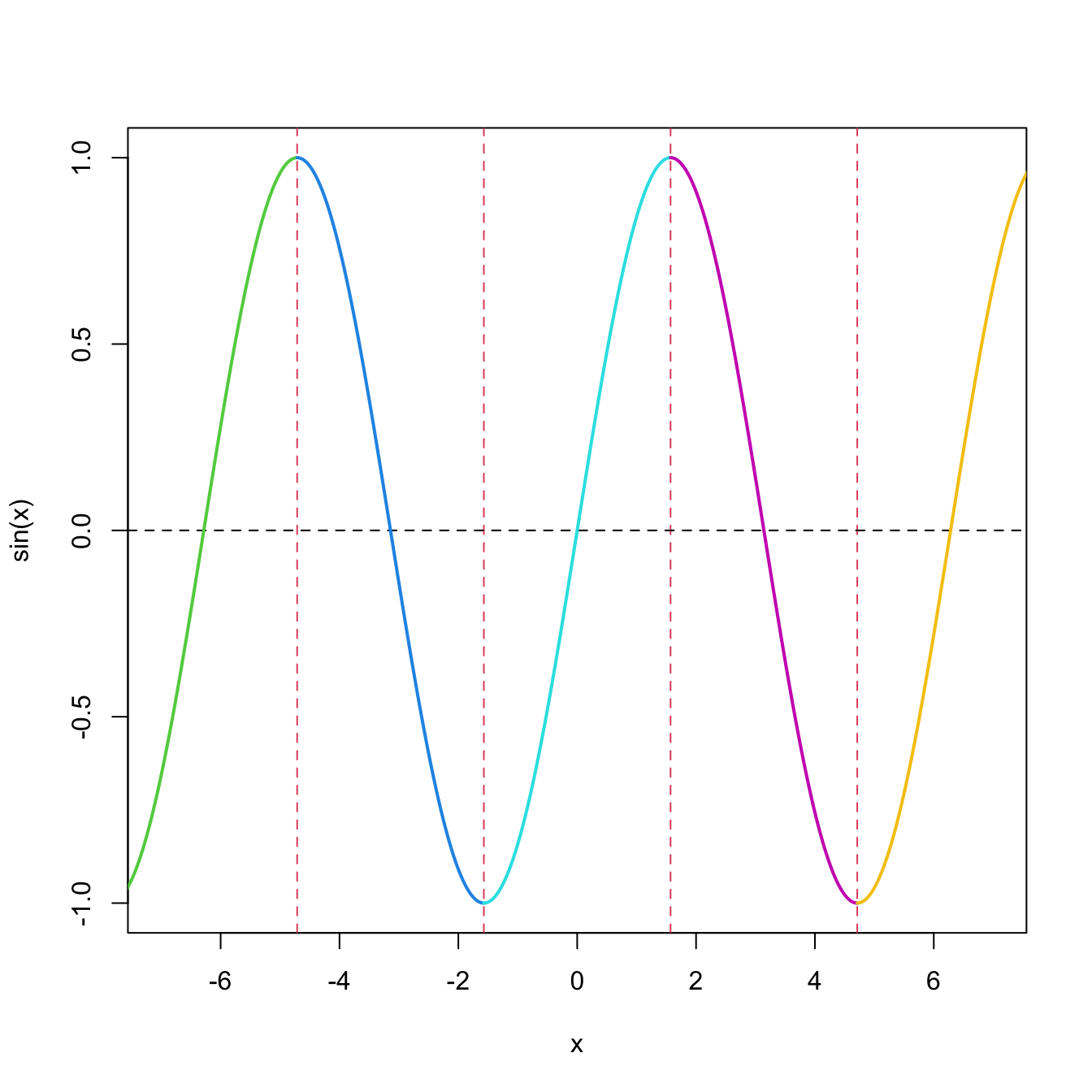
Injective regions of the sine function, marked in different colors separated by vertical dashed lines. There is an infinite number of injective regions.

Figure 1.14: Injective regions of the sine function, marked in different colors separated by vertical dashed lines. There is an infinite number of injective regions.

The functions $g_i:\mathbb{R}^p\rightarrow\mathbb{R}$ are the components of $g=(g_1,\ldots,g_p).$↩︎
Therefore, $g$ has an inverse $g^{-1}.$↩︎
The term $\left\|\frac{\partial g^{-1}(\boldsymbol{y})}{\partial \boldsymbol{y}}\right\|$ is the absolute value of the determinant of the $p\times p$ Jacobian matrix $\frac{\partial g^{-1}(\boldsymbol{y})}{\partial \boldsymbol{y}}=\left(\frac{\partial g_i(\boldsymbol{y})}{\partial y_j}\right)_{ij}.$↩︎
It would not matter if we were leaving out of the partition a finite number of points.↩︎