2.2 Sampling distributions in normal populations

Many rv’s arising in biology, sociology, or economy can be successfully modeled by a normal distribution with mean \(\mu\in\mathbb{R}\) and variance \(\sigma^2\in \mathbb{R}_+.\) This is due to the central limit theorem, a key result in statistical inference that shows that the accumulated effect of a large number of independent rv’s behaves approximately as a normal distribution. Because of this, and the tractability of normal variables, in statistical inference it is usually assumed that the distribution of a rv belongs to the normal family of distributions \(\{\mathcal{N}(\mu,\sigma^2):\mu\in\mathbb{R},\ \sigma^2\in\mathbb{R}_+\},\) where the mean \(\mu\) and the variance \(\sigma^2\) are unknown.

In order to perform inference about \((\mu,\sigma^2),\) a srs \((X_1,\ldots,X_n)\) of \(\mathcal{N}(\mu,\sigma^2)\) is considered. We can compute several statistics using this sample, but we pay special attention to the ones whose values tend to be “similar” to the value of the unknown parameters \((\mu,\sigma^2).\) A statistic of this kind is precisely an estimator. Different kinds of estimators exist depending on the criterion employed to define the “similarity” between the estimator and the parameter to be estimated.

The sample mean \(\bar{X}\) and sample variance \(S^2\) estimators play an important role in statistical inference, since both are “good” estimators of \(\mu\) and \(\sigma^2,\) respectively. As a consequence, it is important to obtain their sampling distributions in order to know their random behaviors. We will do so under the assumption of normal populations.

2.2.1 Sampling distribution of the sample mean

Theorem 2.1 (Distribution of \(\bar{X}\)) Let \((X_1,\ldots,X_n)\) be a srs of size \(n\) of a rv \(\mathcal{N}(\mu,\sigma^2).\) Then, the sample mean \(\bar{X}:=\frac{1}{n}\sum_{i=1}^n X_i\) satisfies \[\begin{align} \bar{X}\sim\mathcal{N}\left(\mu,\frac{\sigma^2}{n}\right). \tag{2.4} \end{align}\]

Proof (Proof of Theorem 2.1). The proof is simple and can actually be done using the mgf through Exercise 2.1 and Proposition 1.5.

Alternatively, assuming that the sum of normal rv’s is another normal (Exercise 2.1), it only remains to compute the resulting mean and variance. The mean is directly obtained from the properties of the expectation, without neither requiring the assumption of normality nor independence:

\[\begin{align*} \mathbb{E}[\bar{X}]=\frac{1}{n}\sum_{i=1}^n \mathbb{E}[X_i] =\frac{1}{n}n\mu=\mu. \end{align*}\]

The variance is obtained by relying only on the hypothesis of independence:

\[\begin{align*} \mathbb{V}\mathrm{ar}[\bar{X}]=\frac{1}{n^2}\sum_{i=1}^n \mathbb{V}\mathrm{ar}[X_i]=\frac{1}{n^2}n\sigma^2=\frac{\sigma^2}{n}. \end{align*}\]

Let’s see some practical applications of this result.

Example 2.7 It is known that the weight (in grams) of liquid that a machine fills into a bottle follows a normal distribution with unknown mean \(\mu\) and standard deviation \(\sigma=25\) grams. From the production of the filling machine along one day, it is obtained a srs of \(n=9\) filled bottles. We want to know what is the probability that the sample mean is closer than \(8\) grams to the real mean \(\mu.\)

If \(X_1,\ldots,X_9\) is the srs that contains the measurements of the nine bottles, then \(X_i\sim\mathcal{N}(\mu,\sigma^2),\) \(i=1,\ldots,n,\) where \(n=9\) and \(\sigma^2=25^2.\) Then, by Theorem 2.1, we have that

\[\begin{align*} \bar{X}\sim\mathcal{N}\left(\mu,\frac{\sigma^2}{n}\right) \end{align*}\]

or, equivalently,

\[\begin{align*} Z=\frac{\bar{X}-\mu}{\sigma/\sqrt{n}}\sim\mathcal{N}(0,1). \end{align*}\]

The desired probability is then

\[\begin{align*} \mathbb{P}(|\bar{X}-\mu|\leq 8) &=\mathbb{P}(-8\leq \bar{X}-\mu\leq 8)\\ &=\mathbb{P}\left(-\frac{8}{\sigma/\sqrt{n}}\leq \frac{\bar{X}-\mu}{\sigma/\sqrt{n}}\leq \frac{8}{\sigma/\sqrt{n}}\right) \\ &=\mathbb{P}(-0.96\leq Z\leq 0.96)\\ &=\mathbb{P}(Z>-0.96)-\mathbb{P}(Z>0.96)\\ &=1-\mathbb{P}(Z>0.96)-\mathbb{P}(Z>0.96) \\ &=1-2\mathbb{P}(Z>0.96)\\ &\approx 1-2\times 0.1685=0.663. \end{align*}\]

The upper-tail probabilities \(\mathbb{P}_Z(Z>k)=1-\mathbb{P}_Z(Z\leq k)\) are given in the \(\mathcal{N}(0,1)\) (outdated) probability tables. More importantly, they can be computed right away with any software package. For example, in R they are obtained with the pnorm() function:

# Computation of P(Z > k)
k <- 0.96
1 - pnorm(k) # 1 - P(Z <= k)
## [1] 0.1685276
pnorm(k, lower.tail = FALSE) # Alternatively
## [1] 0.1685276

Example 2.8 Consider the situation of Example 2.7. How many observations must be included in the sample so that the difference between \(\bar{X}\) and \(\mu\) is smaller than \(8\) grams with a probability \(0.95\)?

The answer is given by the sample size \(n\) that verifies

\[\begin{align*} \mathbb{P}(|\bar{X}-\mu|\leq 8)=\mathbb{P}(-8\leq \bar{X}-\mu\leq 8)=0.95 \end{align*}\]

or, equivalently,

\[\begin{align*} \mathbb{P}\left(-\frac{8}{25/\sqrt{n}}\leq Z\leq \frac{8}{25/\sqrt{n}}\right)=\mathbb{P}(-0.32\sqrt{n}\leq Z\leq 0.32\sqrt{n})=0.95. \end{align*}\]

For a given \(0<\alpha<1,\) we know that the upper \(\alpha/2\)-quantile of a \(Z\sim\mathcal{N}(0,1),\) denoted \(z_{\alpha/2},\) is the quantity such that

\[\begin{align*} \mathbb{P}(-z_{\alpha/2}\leq Z\leq z_{\alpha/2})=1-2\mathbb{P}(Z> z_{\alpha/2})=1-\alpha. \end{align*}\]

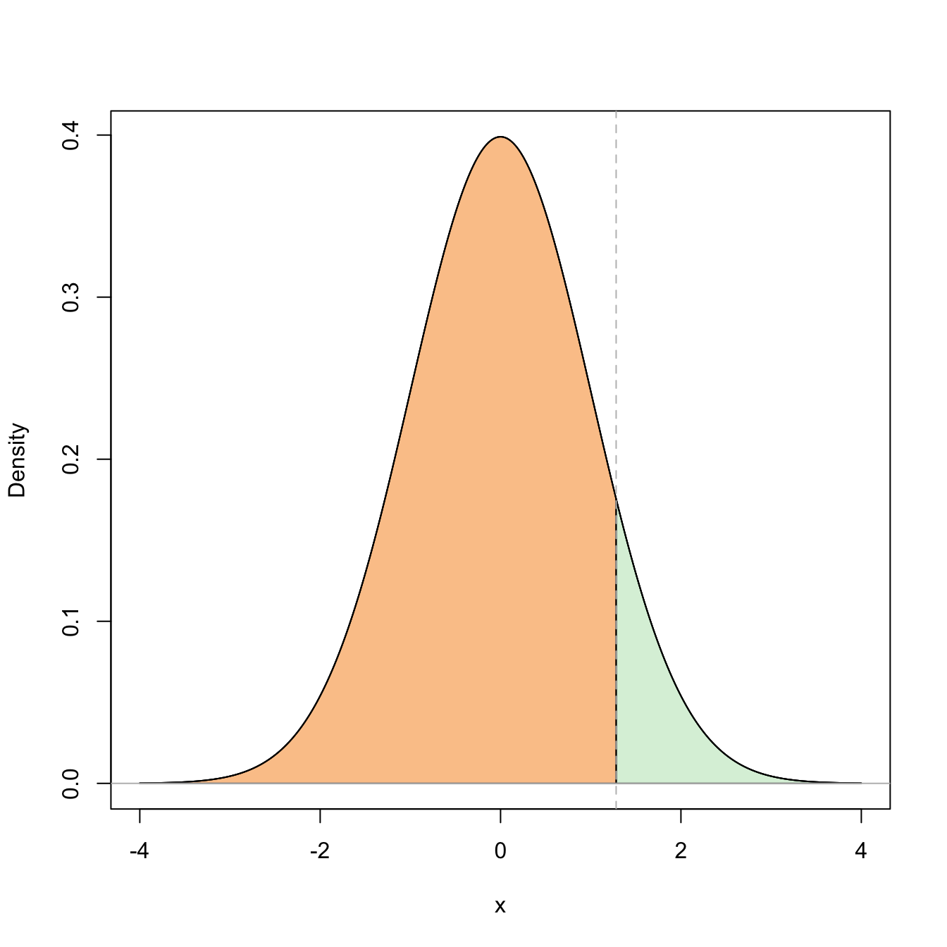
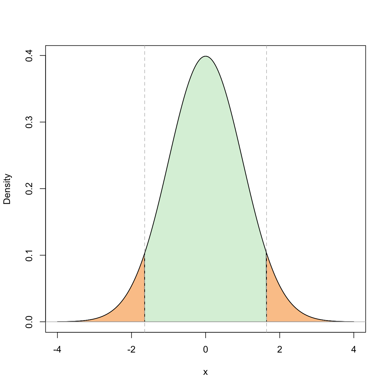
Figure 2.4: Graphical representation of the probabilities \(\mathbb{P}(Z\leq z_{\alpha/2})=1-\alpha\) and \(\mathbb{P}(-z_{\alpha/2}\leq Z\leq z_{\alpha/2})=1-\alpha\) (in green) and their complementaries (in orange) for \(\alpha=0.10\).

Setting \(\alpha=0.05,\) we can easily compute \(z_{0.025}\approx 1.96\) in R through the qnorm() function:

alpha <- 0.05
qnorm(1 - alpha / 2) # LOWER (1 - beta)-quantile = UPPER beta-quantile
## [1] 1.959964
qnorm(alpha / 2, lower.tail = FALSE) # Alternatively, lower.tail = FALSE
## [1] 1.959964
# computes the upper quantile and lower.tail = TRUE (the default) computes the
# lower quantile

Therefore, we set \(0.32\sqrt{n}=z_{0.025}\) and solve for \(n,\) which results in

\[\begin{align*} n=\left(\frac{z_{0.025}}{0.32}\right)^2\approx 37.51. \end{align*}\]

Then, if we take \(n=38,\) we have that

\[\begin{align*} \mathbb{P}(|\bar{X}-\mu|\leq 8)>0.95. \end{align*}\]

2.2.2 Sampling distribution of the sample variance

The sample variance is given by

\[\begin{align*} S^2:=\frac{1}{n}\sum_{i=1}^n (X_i-\bar{X})^2=\frac{1}{n}\sum_{i=1}^n X_i^2-{\bar{X}}^2. \end{align*}\]

The sample quasivariance will also play a relevant role in inference. It is defined by simply replacing \(n\) with \(n-1\) in the factor of \(S^2\):²⁶

\[\begin{align*} S'^2:=\frac{1}{n-1}\sum_{i=1}^n(X_i-\bar{X})^2=\frac{n}{n-1}S^2=\frac{1}{n-1}\sum_{i=1}^n X_i^2-\frac{n}{n-1}{\bar{X}}^2. \end{align*}\]

Before establishing the sampling distributions of \(S^2\) and \(S'^2,\) we obtain in the first place their expectations. For that aim, we start by decomposing the variability of the sample with respect to its expectation \(\mu\) in the following way:

\[\begin{align*} \sum_{i=1}^n(X_i-\mu)^2=\sum_{i=1}^n(X_i-\bar{X})^2+n(\bar{X}-\mu)^2 \end{align*}\]

Taking expectations, we have

\[\begin{align*} n\sigma^2=n\mathbb{E}[S^2]+n\frac{\sigma^2}{n}, \end{align*}\]

and then, solving for the expectation,

\[\begin{align} \mathbb{E}[S^2]=\frac{(n-1)}{n}\,\sigma^2.\tag{2.5} \end{align}\]

Therefore,

\[\begin{align} \mathbb{E}[S'^2]=\frac{n}{n-1}\mathbb{E}[S^2]=\sigma^2.\tag{2.6} \end{align}\]

Recall that this computation does not employ the assumption that of sample normality, hence it is a general fact for \(S^2\) and \(S'^2\) irrespective of the underlying distribution. It also shows that \(S^2\) is not “pointing” towards \(\sigma^2\) but to a slightly smaller quantity, whereas \(S'^2\) is “pointing” directly to \(\sigma^2.\) This observation is related with the bias of an estimator and will be treated in detail in Section 3.1.

In order to compute the sampling distributions of \(S^2\) and \(S'^2,\) it is required to obtain the sampling distribution of the statistic \(\sum_{i=1}^n X_i^2\) when the sample is generated from a \(\mathcal{N}(0,1),\) which will follow a chi-square distribution.

Definition 2.3 (Chi-square distribution) A rv has chi-square distribution with \(\nu\in \mathbb{N}\) degrees of freedom, denoted as \(\chi_{\nu}^2,\) if its distribution coincides with the gamma distribution of shape \(\alpha=\nu/2\) and scale \(\beta=2.\)²⁷ In other words,

\[\begin{align*} \chi_{\nu}^2\stackrel{d}{=}\Gamma(\nu/2,2), \end{align*}\]

with pdf given by

\[\begin{align*} f(x;\nu)=\frac{1}{\Gamma(\nu/2) 2^{\nu/2}}\, x^{\nu/2-1} e^{-x/2}, \quad x>0, \ \nu\in\mathbb{N}. \end{align*}\]

The mean and the variance of a chi-square with \(\nu\) degrees of freedom are²⁸

\[\begin{align} \mathbb{E}[\chi_{\nu}^2]=\nu, \quad \mathbb{V}\mathrm{ar}[\chi_{\nu}^2]=2\nu. \tag{2.7} \end{align}\]

We can observe that a chi-square rv, as any gamma rv, is always positive. Also, their expectation and variance grow accordingly to the degrees of freedom \(\nu.\) When \(\nu\geq 2,\) the pdf attains its global maximum at \(\nu-2.\) If \(\nu=1\) or \(\nu=2,\) the pdf is monotone decreasing. These facts are illustrated in Figure 2.5.

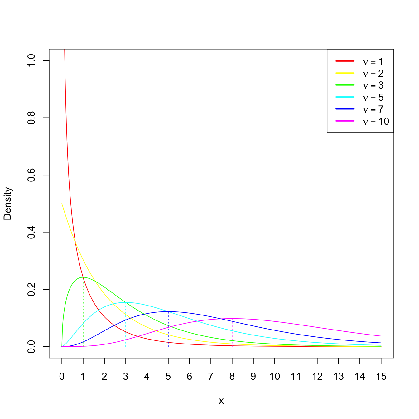
Figure 2.5: \(\chi^2_\nu\) densities for several degrees of freedom \(\nu.\) The dotted lines represent the unique modes of the densities.

The next two propositions are key for obtaining the sampling distribution of \(\sum_{i=1}^n X_i^2,\) given in Corollary 2.1.

Proposition 2.1 If \(X\sim \mathcal{N}(0,1),\) then \(X^2\sim \chi_1^2.\)

Proof (Proof of Proposition 2.1). Rather than using transformations of the pdf, we compute the cdf of the rv \(X^2.\) Since \(X\sim \mathcal{N}(0,1)\) has a symmetric pdf, then

\[\begin{align*} F_{X^2}(y) &=\mathbb{P}_{X^2}(X^2\leq y)=\mathbb{P}\left(-\sqrt{y}\leq X \leq\sqrt{y}\right)=2\mathbb{P}\left(0\leq X \leq \sqrt{y}\right)\\ &=2\int_{0}^{\sqrt{y}} \frac{1}{\sqrt{2\pi}} e^{x^2/2}\,\mathrm{d}x =\int_{0}^y \frac{1}{\sqrt{2\pi}} e^{-u/2} u^{-1/2} \,\mathrm{d}u\\ &=F_{\Gamma(1/2,2)}(y)=F_{\chi^2_1}(y), \; y>0. \end{align*}\]

Proposition 2.2 (Additive property of the chi-square) If \(X_1\sim \chi_n^2\) and \(X_2\sim \chi_m^2\) are independent, then

\[\begin{align*} X_1+X_2\sim \chi_{n+m}^2. \end{align*}\]

Proof (Proof of Proposition 2.2). The chi-square distribution is a particular case of the gamma, so the proof follows immediately using Exercise 1.21.

Corollary 2.1 Let \(X_1,\ldots,X_n\) be independent rv’s distributed as \(\mathcal{N}(0,1).\) Then,

\[\begin{align*} \sum_{i=1}^n X_i^2\sim \chi_n^2. \end{align*}\]

Proof. The proof follows directly from Propositions 2.1 and 2.2.

The last result is sometimes employed for directly defining the chi-square rv with \(\nu\) degrees of freedom as the sum of \(\nu\) independent squared \(\mathcal{N}(0,1)\) rv’s. In this way, the degrees of freedom represent the number of terms in the sum.

Example 2.9 If \((Z_1,\ldots,Z_6)\) is a srs of a standard normal, find a number \(b\) such that

\[\begin{align*} \mathbb{P}\left(\sum_{i=1}^6 Z_i^2\leq b\right)=0.95. \end{align*}\]

We know from Corollary 2.1 that

\[\begin{align*} \sum_{i=1}^6 Z_i^2\sim \chi_6^2. \end{align*}\]

Then, \(b\approx 12.59\) corresponds to the upper \(\alpha\)-quantile of a \(\chi^2_{\nu},\) denoted as \(\chi^2_{\nu;\alpha}.\) Here, \(\alpha=0.05\) and \(\nu=6.\) The quantiles \(\chi^2_{6;0.05}\) can be computed by calling the qchisq() function in R:

alpha <- 0.05
qchisq(1 - alpha, df = 6) # df stands for the degrees of freedom
## [1] 12.59159
qchisq(alpha, df = 6, lower.tail = FALSE) # Alternatively
## [1] 12.59159

The final result of this section is the famous Fisher’s Theorem, which delivers the sampling distribution of \(S^2\) and \(S'^2,\) and their independence²⁹ with respect to \(\bar{X}.\)

Theorem 2.2 (Fisher's Theorem) If \((X_1,\ldots,X_n)\) is a srs of a \(\mathcal{N}(\mu,\sigma^2)\) rv, then \(S^2\) and \(\bar{X}\) are independent, and

\[\begin{align*} \frac{nS^2}{\sigma^2}=\frac{(n-1)S'^2}{\sigma^2}\sim\chi_{n-1}^2. \end{align*}\]

Proof (Proof of Theorem 2.2). We apply Theorem 2.6 given in the Appendix for \(p=1,\) in such a way that

\[\begin{align*} nS^2=\sum_{i=1}^n X_i^2-(\sqrt{n}\bar{X})^2=\sum_{i=1}^n X_i^2-\boldsymbol{c}_1' X, \end{align*}\]

for \(\boldsymbol{c}_1=(1/\sqrt{n},\ldots,1/\sqrt{n})'\) and \(\boldsymbol{X}=(X_1,\ldots,X_n)'.\) Therefore, by such theorem, \(S^2\) is independent of \(\bar{X},\) and \(\frac{nS^2}{\sigma^2}\sim \chi_{n-1}^2.\)

Example 2.10 Assume that we have a srs made of 10 bottles from the filling machine of Example 2.7 where \(\sigma^2=625.\) Find a pair of values \(b_1\) and \(b_2\) such that

\[\begin{align*} \mathbb{P}(b_1\leq S'^2\leq b_2)=0.90. \end{align*}\]

We know from Theorem 2.2 that \(\frac{(n-1)S'^2}{\sigma^2}\sim\chi_{n-1}^2.\) Therefore, multiplying by \((n-1)\) and dividing by \(\sigma^2\) in the previous probability, we get

\[\begin{align*} \mathbb{P}(b_1\leq S'^2\leq b_2)&=\mathbb{P}\left(\frac{(n-1)b_1}{\sigma^2}\leq \frac{(n-1)S'^2}{\sigma^2} \leq \frac{(n-1)b_2}{\sigma^2}\right)\\ &=\mathbb{P}\left(\frac{9b_1}{625}\leq \chi_9^2 \leq \frac{9b_2}{625}\right). \end{align*}\]

Set \(a_1=\frac{9b_1}{625}\) and \(a_2=\frac{9b_2}{625}.\) A possibility is to select:

• \(a_1\) such that the cumulative probability to its left (right) is \(0.05\) (\(0.95\)). This corresponds to the upper \((1-\alpha/2)\)-quantile, \(\chi^2_{\nu;1-\alpha/2},\) with \(\alpha=0.10\) (because \(1-\alpha=0.90\)).
• \(a_2\) such that the cumulative probability to its right is \(0.05.\) This corresponds to the upper \(\alpha/2\)-quantile, \(\chi^2_{\nu;\alpha/2}.\)

Recall that, unlike in the situation of Example 2.8, the pdf of a chi-square is not symmetric, and hence \(\chi^2_{\nu;1-\alpha}\neq -\chi^2_{\nu;\alpha}\) (for the normal we had that \(z_{1-\alpha}= -z_{\alpha}\) and therefore we only cared about \(z_{\alpha}\)).

We can compute \(a_1=\chi^2_{9;0.95}\) and \(a_2=\chi^2_{9;0.05}\) by employing the function qchisq():

alpha <- 0.10
qchisq(1 - alpha / 2, df = 9, lower.tail = FALSE) # a1
## [1] 3.325113
qchisq(alpha / 2, df = 9, lower.tail = FALSE) # a2
## [1] 16.91898

Then, \(a_1\approx3.325\) and \(a_2\approx16.919,\) so the asked values are \(b_1\approx3.325\times 625/9=230.903\) and \(b_2\approx 16.919\times 625 / 9=1174.931.\)

2.2.3 Student’s \(t\) distribution

Definition 2.4 (Student’s \(t\) distribution) Let \(X\sim \mathcal{N}(0,1)\) and \(Y\sim \chi_{\nu}^2\) be independent rv’s. The distribution of the rv

\[\begin{align*} T=\frac{X}{\sqrt{Y/\nu}} \end{align*}\]

is the Student’s \(t\) distribution with \(\nu\) degrees of freedom.³⁰

The pdf of the Student’s \(t\) distribution is (see the Exercise 2.22)

\[\begin{align*} f(t;\nu)=\frac{\Gamma\left(\frac{\nu+1}{2}\right)}{\sqrt{\nu \pi}\,\Gamma\left(\frac{\nu}{2}\right)}\left(1+\frac{t^2}{\nu}\right)^{-(\nu+1)/2},\quad t\in \mathbb{R}. \end{align*}\]

We can see that the density is symmetric with respect to zero. When \(\nu>1\)³¹, its expectation is \(\mathbb{E}[T]=0\) and, when \(\nu>2,\) its variance is \(\mathbb{V}\mathrm{ar}[T]=\nu/(\nu-2)>1.\) This means that for \(\nu>2,\) \(T\) has a larger variability than the standard normal. However, the differences between a \(t_{\nu}\) and a \(\mathcal{N}(0,1)\) vanish as \(\nu\to\infty,\) as it can be seen in Figure 2.6.

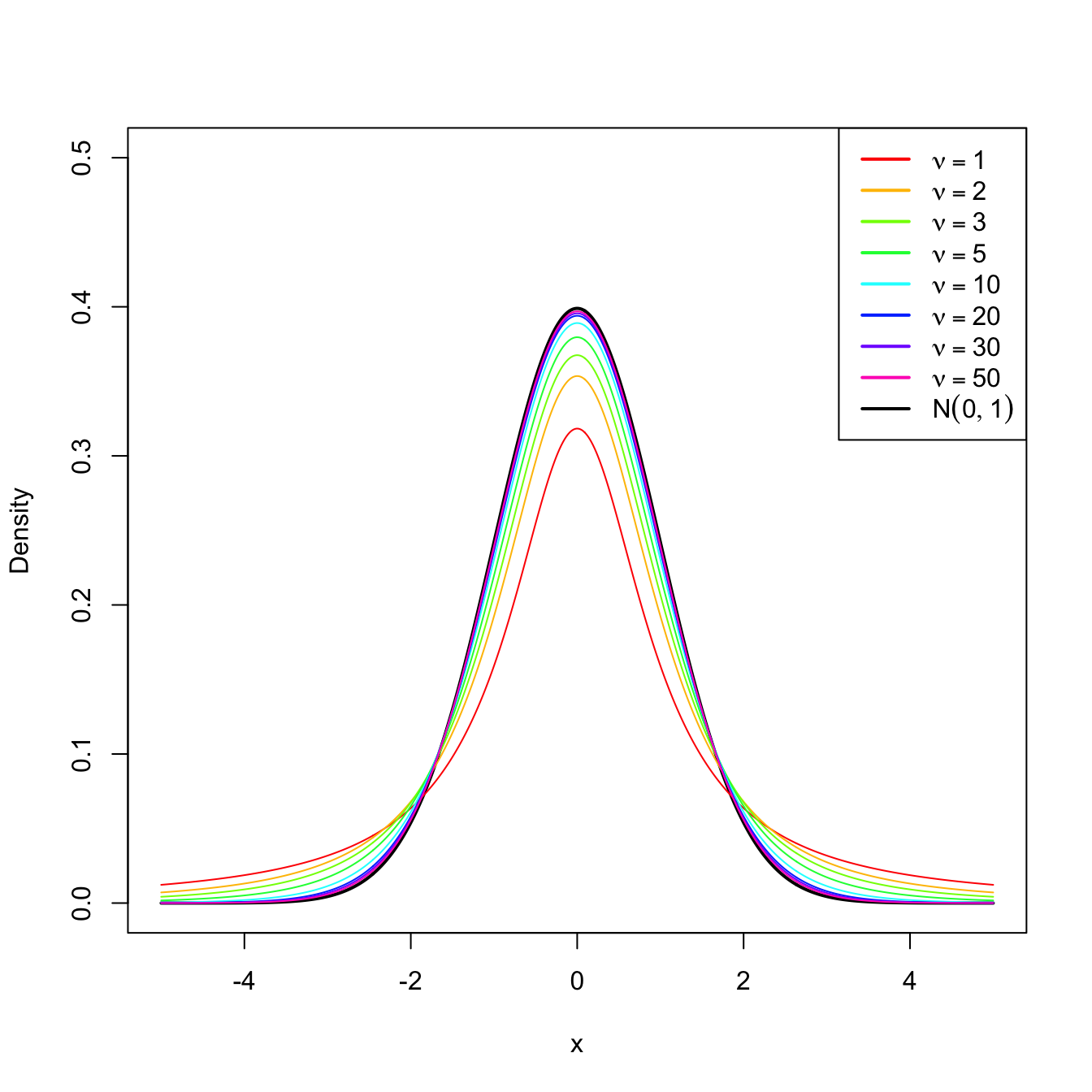
Figure 2.6: \(t_\nu\) densities for several degrees of freedom \(\nu.\) Observe the convergence to a \(\mathcal{N}(0,1)\) as \(\nu\to\infty.\)

Theorem 2.3 (Student's Theorem) Let \((X_1,\ldots,X_n)\) be a srs of a \(\mathcal{N}(\mu,\sigma^2)\) rv. Let \(\bar{X}\) and \(S'^2\) be the sample mean and quasivariance, respectively. Then,

\[\begin{align*} T=\frac{\bar{X}-\mu}{S'/\sqrt{n}}\sim t_{n-1}. \end{align*}\]

and the statistic \(T\) is referred to as the (Student’s) \(T\) statistic.

Proof (Proof of Theorem 2.3). From Theorem 2.1, we can deduce that

\[\begin{align} \frac{\bar{X}-\mu}{\sigma/\sqrt{n}}\sim \mathcal{N}(0,1).\tag{2.8} \end{align}\]

On the other hand, by Theorem 2.2 we know that

\[\begin{align} \frac{(n-1)S'^2}{\sigma^2}\sim \chi_{n-1}^2,\tag{2.9} \end{align}\]

and that (2.9) is independent of (2.8). Therefore, dividing (2.8) by the square root of (2.9) divided by its degrees of freedom, we obtain a rv with Student’s \(t\) distribution:

\[\begin{align*} T=\frac{\sqrt{n}\, \frac{\bar{X}-\mu}{\sigma}}{\sqrt{\frac{(n-1)S'^2}{\sigma^2}/(n-1)}}=\frac{\bar{X}-\mu}{S'/\sqrt{n}}\sim t_{n-1}. \end{align*}\]

Example 2.11 The resistance to electric tension of a certain kind of wire is distributed according to a normal with mean \(\mu\) and variance \(\sigma^2,\) both unknown. Six segments of the wire are selected at random and measured their resistance, being these measurements \(X_1,\ldots,X_6.\) Find the approximate probability that the difference between \(\bar{X}\) and \(\mu\) is less than \(2S'/\sqrt{n}\) units.

We want to compute the probability

\[\begin{align*} \mathbb{P}&\left(-\frac{2S'}{\sqrt{n}}\leq \bar{X}-\mu\leq\frac{2S'}{\sqrt{n}}\right)=\mathbb{P}\left(-2\leq \sqrt{n}\frac{\bar{X}-\mu}{S'}\leq 2\right)\\ &\quad=\mathbb{P}(-2\leq T\leq 2)=1-2\mathbb{P}(T\leq -2). \end{align*}\]

From Theorem 2.3, we know that \(T\sim t_5.\) The probabilities \(\mathbb{P}(t_\nu\leq x)\) can be computed with pt(x, df = nu):

pt(-2, df = 5)
## [1] 0.05096974

Therefore, the probability is approximately \(1-2\times 0.051=0.898.\)

2.2.4 Snedecor’s \(\mathcal{F}\) distribution

Definition 2.5 (Snedecor’s \(\mathcal{F}\) distribution) Let \(X_1\) and \(X_2\) be chi-square rv’s with \(\nu_1\) and \(\nu_2\) degrees of freedom, respectively. If \(X_1\) and \(X_2\) are independent, then the rv

\[\begin{align*} F=\frac{X_1/\nu_1}{X_2/\nu_2} \end{align*}\]

is said to have an Snedecor’s \(\mathcal{F}\) distribution with \(\nu_1\) and \(\nu_2\) degrees of freedom, which is represented as \(\mathcal{F}_{\nu_1,\nu_2}.\)

Remark. It can be seen that \(\mathcal{F}_{1,\nu}\) coincides with \(t_{\nu}^2.\)

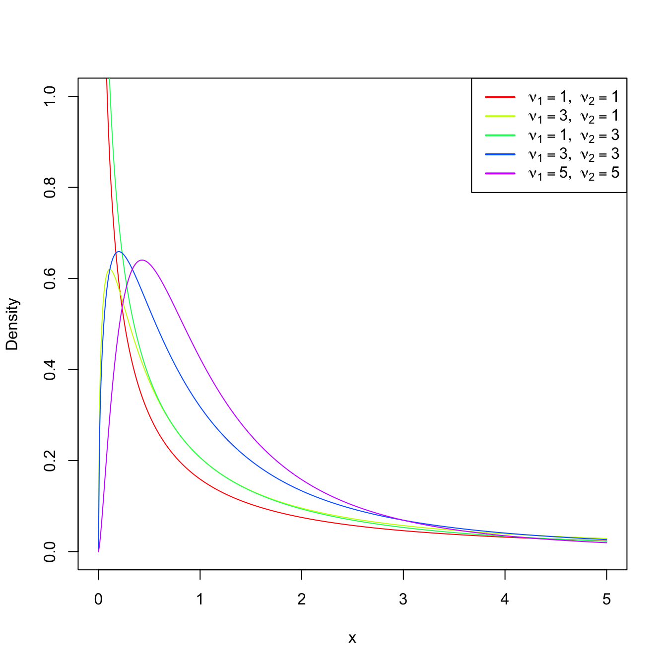
Figure 2.7: \(\mathcal{F}_{\nu_1,\nu_2}\) densities for several degrees of freedom \(\nu_1\) and \(\nu_2.\)

Theorem 2.4 (Sampling distribution of the ratio of quasivariances) Let \((X_1,\ldots,X_{n_1})\) be a srs from a \(\mathcal{N}(\mu_1,\sigma_1^2)\) and let \(S_1'^2\) be its sample quasivariance. Let \((Y_1,\ldots,Y_{n_2})\) be another srs, independent from the previous one, from a \(\mathcal{N}(\mu_2,\sigma_2^2)\) and with sample quasivariance \(S_2'^2.\) Then,

\[\begin{align*} F=\frac{S_1'^2/\sigma_1^2}{S_2'^2/\sigma_2^2}\sim\mathcal{F}_{n_1-1,n_2-1}. \end{align*}\]

Proof (Proof of Theorem 2.4). The proof is straightforward from the independence of both samples, the application of Theorem 2.2 and the definition of Snedecor’s \(\mathcal{F}\) distribution, since

\[\begin{align*} F=\frac{\frac{(n_1-1)S_1'^2}{\sigma_1^2}/(n_1-1)}{\frac{(n_2-1)S_2'^2}{\sigma_2^2}/(n_2-1)}=\frac{S_1'^2/\sigma_1^2}{S_2'^2/\sigma_2^2}\sim\mathcal{F}_{n_1-1,n_2-1}. \end{align*}\]

Example 2.12 If we take two independent srs’s of sizes \(n_1=6\) and \(n_2=10\) from two normal populations with the same (but unknown) variance \(\sigma^2,\) find the number \(b\) such that

\[\begin{align*} \mathbb{P}\left(\frac{S_1'^2}{S_2'^2}\leq b\right)=0.95. \end{align*}\]

We have that

\[\begin{align*} \mathbb{P}\left(\frac{S_1'^2}{S_2'^2}\leq b\right)=0.95\iff \mathbb{P}\left(\frac{S_1'^2}{S_2'^2}> b\right)=0.05. \end{align*}\]

By Theorem 2.4, we know that

\[\begin{align*} \frac{S_1'^2/\sigma_1^2}{S_2'^2/\sigma_2^2}=\frac{S_1'^2}{S_2'^2}\sim\mathcal{F}_{5,9}. \end{align*}\]

Therefore, we look for the upper \(\alpha\)-quantile \(\mathcal{F}_{\nu_1,\nu_2;\alpha}\) such that \(\mathbb{P}(\mathcal{F}_{\nu_1,\nu_2}>\mathcal{F}_{\nu_1,\nu_2;\alpha})=\alpha,\) for \(\alpha=0.05,\) \(\nu_1=5,\) and \(\nu_2=9.\) This can be obtained with the function qf(), which provides \(b=:\mathcal{F}_{5,9;0.05}\):

qf(0.05, df1 = 5, df2 = 9, lower.tail = FALSE)
## [1] 3.481659

References

Kagan, A. M., Y. V. Linnik, and C. R. Rao. 1973. Characterization Problems in Mathematical Statistics. Wiley Series in Probability and Mathematical Statistics. New York: John Wiley & Sons.

---

26. This correction is known as Bessel’s correction.↩︎

27. Recall the definition of the gamma distribution given in Example 1.21.↩︎

28. See Example 1.23.↩︎

29. This property is actually unique of the normal distribution. That is, the normal distribution is the only distribution for which \(S^2\) and \(\bar{X}\) are independent! This characterization of the normal distribution can be seen in Section 4.2 of Kagan, Linnik, and Rao (1973) (the book contains many other characterizations of the normal and other distributions).↩︎

30. When \(\nu=1,\) this distribution is known as the Cauchy distribution with null location and unit scale. See Exercise 2.4.↩︎

31. When \(\nu=1\) the expectation does not exist! The same happens for the variance when \(\nu=1,2.\)↩︎