1.2 Random variables

The random variable concept allows transforming the sample space $\Omega$ of a random experiment into a set with good mathematical properties, such as the real numbers $\mathbb{R},$ effectively forgetting spaces like $\Omega=\{\mathrm{H},\mathrm{T}\}.$

Definition 1.13 (Random variable) Let $(\Omega,\mathcal{A})$ be measurable space. Let $\mathcal{B}$ be the Borel $\sigma$-algebra over $\mathbb{R}.$ A random variable (rv) is a mapping $X:\Omega\rightarrow \mathbb{R}$ that is measurable, that is, that verifies

$$\begin{align*} \forall B\in\mathcal{B}, \quad X^{-1}(B)\in\mathcal{A}, \end{align*}$$

with $X^{-1}(B)=\{\omega\in\Omega: X(\omega)\in B\}.$

The adjective measurable for the mapping $X:\Omega\rightarrow \mathbb{R}$ simply means that any Borelian $B$ has been generated through $X$ with a set ($X^{-1}(B)$) that belongs to $\mathcal{A}$ and therefore measure can be assigned to it.

A random variable transforms a measurable space $(\Omega,\mathcal{A})$ into another measurable space with a more convenient mathematical framework, $(\mathbb{R},\mathcal{B}),$ whose $\sigma$-algebra is the one generated by the class of intervals. The measurability condition of the random variable allows to transfer the probability of any subset $A\in\mathcal{A}$ to the probability of a subset $B\in\mathcal{B},$ where $B$ is precisely the image of $A$ through the random variable $X.$ The concept of random variable reveals itself as a key translator: it allows transferring the randomness “produced” by the concept of a random experiment with sample space $\Omega$ to the mathematical-friendly $(\mathbb{R},\mathcal{B}).$ After this transfer is done, we do not require dealing with $(\Omega,\mathcal{A})$ anymore and we can focus on $(\mathbb{R},\mathcal{B})$ (yet $(\Omega,\mathcal{A})$ is always underneath).³

Remark. The space $(\Omega,\mathcal{A})$ is dependent on $\xi.$ However, $(\mathbb{R},\mathcal{B})$ is always the same space, irrespective of $\xi$!

Example 1.7 For the experiments given in Example 1.1, the next are random variables:

1. A possible random variable for the measurable space $$\begin{align*} \Omega=\{\mathrm{H},\mathrm{T}\}, \quad \mathcal{A}=\{\emptyset,\{\mathrm{H}\},\{\mathrm{T}\},\Omega\}, \end{align*}$$ is $$\begin{align*} X(\omega):=\begin{cases} 1, & \mathrm{if}\ \omega=\mathrm{H},\\ 0, & \mathrm{if}\ \omega=\mathrm{T}. \end{cases} \end{align*}$$ We can call this random variable “Number of heads when tossing a coin”. Indeed, this is a random variable, since for any subset $B\in\mathcal{B},$ it holds:
   • If $0,1\in B,$ then $X^{-1}(B)=\Omega\in \mathcal{A}.$
   • If $0\in B$ but $1\notin B,$ then $X^{-1}(B)=\{\mathrm{T}\}\in \mathcal{A}.$
   • If $1\in B$ but $0\notin B,$ then $X^{-1}(B)=\{\mathrm{H}\}\in \mathcal{A}.$
   • If $0,1\notin B,$ then $X^{-1}(B)=\emptyset\in \mathcal{A}.$
2. For the measurable space $(\Omega,\mathcal{P}(\Omega)),$ where $\Omega=\mathbb{N}_0,$ since the sample space is already contained in $\mathbb{R},$ an adequate random variable is $X_1(\omega):=\omega.$ Indeed, $X_1$ is a random variable, because for $B\in\mathcal{B},$ the set $$\begin{align*} X_1^{-1}(B)=\{\omega\in \mathbb{N}_0: X_1(\omega)=\omega\in B\} \end{align*}$$ is the set of natural numbers (including zero) that belong to $B.$ But any countable set of natural numbers belongs to $\mathcal{P}(\Omega),$ as this $\sigma$-algebra contains all the subsets of $\mathbb{N}_0.$ Therefore, $X_1=$ “Number of car accidents within a day in Spain” is a random variable. Another possible random variable is the one that indicates whether there is at least one car accident, and is given by $$\begin{align*} X_2(\omega):=\begin{cases} 1, & \mathrm{if}\ \omega\in \mathbb{N}, \\ 0, & \mathrm{if} \ \omega=0. \end{cases} \end{align*}$$ Indeed, $X_2$ is a random variable, since for $B\in\mathcal{B}$:
   • If $0,1\in B,$ then $X_2^{-1}(B)=\Omega\in \mathcal{P}(\Omega).$
   • If $1\in B$ but $0\notin B,$ then $X_2^{-1}(B)=\mathbb{N}\in \mathcal{P}(\Omega).$
   • If $0\in B$ but $1\notin B,$ then $X_2^{-1}(B)=\{0\}\in \mathcal{P}(\Omega).$
   • If $0,1\notin B,$ then $X_2^{-1}(B)=\emptyset\in \mathcal{P}(\Omega).$
3. As in the previous case, for the measurable space $(\Omega,\mathcal{B}_{\Omega}),$ where $\Omega=[m,\infty),$ a random variable is $X_1(\omega):=\omega,$ since for $B\in \mathcal{B},$ we have $$\begin{align*} X_1^{-1}(B)=\{\omega\in[m,\infty): X_1(\omega)=\omega\in B\}=[m,\infty)\cap B\in \mathcal{B}_{\Omega}. \end{align*}$$ $X_1$ is therefore a random variable that corresponds to the “Weight of a pedestrian between 20 and 40 years old”. Another possible random variable is $$\begin{align*} X_2(\omega):=\begin{cases} 1, & \mathrm{if}\ \omega \geq 65,\\ 0, & \mathrm{if}\ \omega<65, \end{cases} \end{align*}$$ which corresponds to the concept “Weight of at least 65 kilograms”.

Example 1.8 Let $\xi=$ “Draw a point at random from $\Omega=\{(x,y)'\in\mathbb{R}^2:x^2+y^2\leq 1\}$”. Then, $\omega=(x,y)'\in\Omega$ and we can define the random variable $X:=$ “Distance to the center of $\Omega$” as $X(\omega)=\sqrt{x^2+y^2}.$ It can be seen (but it is technical) that indeed $X$ is a proper random variable for the measurable space $(\Omega,\mathcal{B}^2_\Omega),$ where $\mathcal{B}^2=\{A_1\times A_2:A_1,A_2\in\mathcal{B}\}.$

The induced probability of a random variable is the probability function defined over subsets of $\mathbb{R}$ that preserves the probabilities of the original events of $\Omega.$ This gives the final touch for completely translating the probability space $(\Omega,\mathcal{A},\mathbb{P})$ to the probability space $(\mathbb{R},\mathcal{B},\mathbb{P}_X),$ which is much more manageable.

Definition 1.14 (Induced probability of a rv) Let $\mathcal{B}$ be the Borel $\sigma$-algebra over $\mathbb{R}.$ The induced probability of the rv $X$ is the function $\mathbb{P}_X:\mathcal{B}\rightarrow \mathbb{R}$ defined as

$$\begin{align*} \mathbb{P}_X(B):=\mathbb{P}(X^{-1}(B)), \quad \forall B\in \mathcal{B}. \end{align*}$$

Example 1.9 Consider the probability function $\mathbb{P}_1$ defined in Example 1.4 and the random variable $X$ defined in part a in Example 1.7. For $B\in\mathcal{B},$ the induced probability of $X$ is described in the following way:

• If $0,1\in B,$ then $\mathbb{P}_{1X}(B)=\mathbb{P}_1(X^{-1}(B))=\mathbb{P}_1(\Omega)=1.$
• If $0\in B$ but $1\notin B,$ then $\mathbb{P}_{1X}(B)=\mathbb{P}_1(X^{-1}(B))=\mathbb{P}_1(\{\mathrm{T}\})=1/2.$
• If $1\in B$ but $0\notin B,$ then $\mathbb{P}_{1X}(B)=\mathbb{P}_1(X^{-1}(B))=\mathbb{P}_1(\{\mathrm{H}\})=1/2.$
• If $0,1\notin B,$ then $\mathbb{P}_{1X}(B)=\mathbb{P}_1(X^{-1}(B))=\mathbb{P}_1(\emptyset)=0.$

Therefore, the induced probability by $X$ is

$$\begin{align*} \mathbb{P}_{1X}(B)=\begin{cases} 0, & \mathrm{if}\ 0,1\notin B,\\ 1/2, & \text{if $0$ or $1$ are in $B$},\\ 1, & \mathrm{if}\ 0,1\in B. \end{cases} \end{align*}$$

Particularly, we have the following probabilities:

• $\mathbb{P}_{1X}(\{0\})=\mathbb{P}_1(X=0)=1/2.$
• $\mathbb{P}_{1X}((-\infty,0])=\mathbb{P}_1(X\leq 0)=1/2.$
• $\mathbb{P}_{1X}((0,1])=\mathbb{P}_1(0< X\leq 1)=1/2.$

Example 1.10 For the probability function $\mathbb{P}$ defined in Example 1.5 and the random variable $X_1$ defined in part b in Example 1.7, the induced probability by the random variable $X_1$ is described in the following way. Let $B\in\mathcal{B}$ be such that $\mathbb{N}_0\cap B=\{a_1,a_2,\ldots,a_p\}.$ Then:

$$\begin{align*} \mathbb{P}_{X_1}(B)&=\mathbb{P}(X_1^{-1}(B))=\mathbb{P}_1(\mathbb{N}_0\cap B)\\ &=\mathbb{P}(\{a_1,a_2,\ldots,a_p\})=\sum_{i=1}^p \mathbb{P}(\{a_i\}). \end{align*}$$

In practice, we will not need to do compute what is the probability induced $\mathbb{P}_X$ of a random variable $X$ that is based on a random experiment $\xi.$ We will take a shortcut: directly specify $\mathbb{P}_X$ via a probability model, and forget about the conceptual pillars on which $X$ and $\mathbb{P}_X$ are built (the random experiment $\xi$ and the probability space $(\Omega,\mathcal{A},\mathbb{P})$). For introducing probability models, we need to distinguish first among the two main types of random variables: discrete and continuous.

1.2.1 Types of random variables

Before diving into the specifics of discrete and continuous variables we introduce the common concept of cumulative distribution function of a random variable $X.$

Definition 1.15 (Cumulative distribution function) The cumulative distribution function (cdf) of a random variable $X$ is the function $F_X:\mathbb{R}\rightarrow [0,1]$ defined as

$$\begin{align*} F_X(x):=\mathbb{P}_X((-\infty,x]), \quad \forall x\in \mathbb{R}. \end{align*}$$

We will denote $\mathbb{P}(X\leq x):=\mathbb{P}_X((-\infty,x])$ for simplicity.

Remark. The cdf is properly defined since $(-\infty,x]\in\mathcal{B},$ so $\mathbb{P}_X((-\infty,x])=\mathbb{P}(X^{-1}(-\infty,x])$ and since $X$ is measurable (from the definition of a random variable), then $X^{-1}(-\infty,x]\in\mathcal{A}$ and $\mathbb{P}(X^{-1}(-\infty,x])$ is well-defined.

The following properties are easy to check.

Proposition 1.3 (Properties of the cdf)

1. The cdf is monotonically non-decreasing, that is, $$\begin{align*} x<y \implies F_X(x)\leq F_X(y). \end{align*}$$
2. Let $a,b\in\mathbb{R}$ such that $a<b.$ Then, $$\begin{align*} \mathbb{P}(a<X\leq b)=F_X(b)-F_X(a). \end{align*}$$
3. $\lim_{x\to-\infty} F(x)=0.$
4. $\lim_{x\to\infty} F(x)=1.$
5. $F_X$ is right-continuous.⁴
6. The set of points where $F_X$ is discontinuous is finite or countable.

Definition 1.16 (Discrete random variable) A random variable $X$ is discrete if its range (or image set) $R_X:=\{x\in \mathbb{R}: x=X(\omega)\ \text{for some} \ \omega\in \Omega\}$ is finite or countable.

Example 1.11 Among the random variables defined in Example 1.7, the ones from parts a and b are discrete, and so is $X_2$ from part c.

In the case of discrete random variables, we can define a function that gives, in particular, the probabilities of the individual points of its range $R_X.$

Definition 1.17 (Probability mass function) The probability mass function (pmf) of a discrete random variable $X$ is the function $p_X:\mathbb{R}\rightarrow [0,1]$ defined by

$$\begin{align*} p_X(x):=\mathbb{P}_X(\{x\}), \quad \forall x\in \mathbb{R}. \end{align*}$$

We will denote $\mathbb{P}(X=x):=\mathbb{P}_X(\{x\})$ for simplicity.

With the terminology “distribution of a discrete random variable $X$” we refer to either the probability function induced by $X,$ $\mathbb{P}_X,$ the cdf $F_X,$ or the pmf $p_X.$ The motivation for this abuse of notation is that any of these functions completely determine the random behavior of $X.$

Definition 1.18 (Continuous random variable) A continuous random variable $X$ (more precisely denoted absolutely continuous⁵) is the one whose cdf $F_X$ is expressible as

$$\begin{align} F_X(x)=\int_{-\infty}^x f_X(t)\,\mathrm{d}t,\quad\forall x\in\mathbb{R},\tag{1.2} \end{align}$$

where $f_X:\mathbb{R}\rightarrow[0,\infty).$ The function $f_X$ is the probability density function (pdf) of $X.$ Sometimes the pdf is simply referred to as the density function.

Example 1.12 The random variable $X_1=$ “Weight of a pedestrian between 20 and 40 years old”, defined in part c of Example 1.7, is continuous.

The pdf is called like that because, for any $x\in\mathbb{R},$ it measures the density of the probability of an infinitesimal interval centered at $x.$

Proposition 1.4 (Properties of the pdf)

1. $F_X'(x)=f_X(x)$ for almost all $x\in\mathbb{R}.$⁶
2. $f$ is such that $$\begin{align*} \int_{-\infty}^{\infty} f_X(t)\,\mathrm{d}t=1. \end{align*}$$
3. For $A\in\mathcal{B},$ $\mathbb{P}(X\in A)=\int_{A} f_X(t)\,\mathrm{d}t.$⁷

As in the discrete case, a continuous random variable $X$ is fully determined by either the induced probability function $\mathbb{P}_X,$ the cdf $F_X,$ or the pdf $f_X.$ Therefore, whenever we refer to the “distribution of a random variable”, we may be referring to any of these functions.

Remark. Observe that, for a discrete random variable $X,$ the cdf $F_X$ can be obtained by the pmf $p_X$ in an analogous way to (1.2):

$$\begin{align*} F_X(x)=\sum_{\{x_i\in\mathbb{R}:p_X(x_i)>0,\,x_i\leq x\}}p_X(x_i). \end{align*}$$

Remark. Recall that the cdf accumulates probability irrespective of the type of the random variable. It does not assign probability to specific values of $X;$ this is a type-dependent operation:

• If $X$ is discrete, the assignment of probability is done by the pmf $p_X.$ The values that $X$ can take with positive probability are called atoms.
• If $X$ is continuous, the assignment of infinitesimal probability is done by the pdf $f_X.$ There are no atoms in a continuous random variable, since $\mathbb{P}(X=x)=\int_x^xf_X(t)\,\mathrm{d}t=0$ for any $x\in\mathbb{R}.$

We will write $X\sim F$ to denote that the random variable $X$ has cdf $F.$ In other words, the symbol “$\sim$” (tilde) stands for “distributed as”. Sometimes $F$ is denoted by a more evocative symbol representing the distribution, as illustrated in the following examples.

Example 1.13 (Uniform (discrete)) The random variable $X\sim\mathcal{U}(\{1,\ldots,N\})$ is such that its pmf is

$$\begin{align*} p(x;N)=\frac{1}{N},\quad x=1,\ldots,N. \end{align*}$$

Example 1.14 (Poisson model) The random variable $X\sim\mathrm{Pois}(\lambda),$ $\lambda>0$ (intensity parameter), is such that its pmf is

$$\begin{align*} p(x;\lambda)=\frac{e^{-\lambda}\lambda^x}{x!},\quad x=0,1,2,\ldots \end{align*}$$

The points $\{0,1,2,\ldots\}$ are the atoms of $X.$ This probability model is useful to model counts.

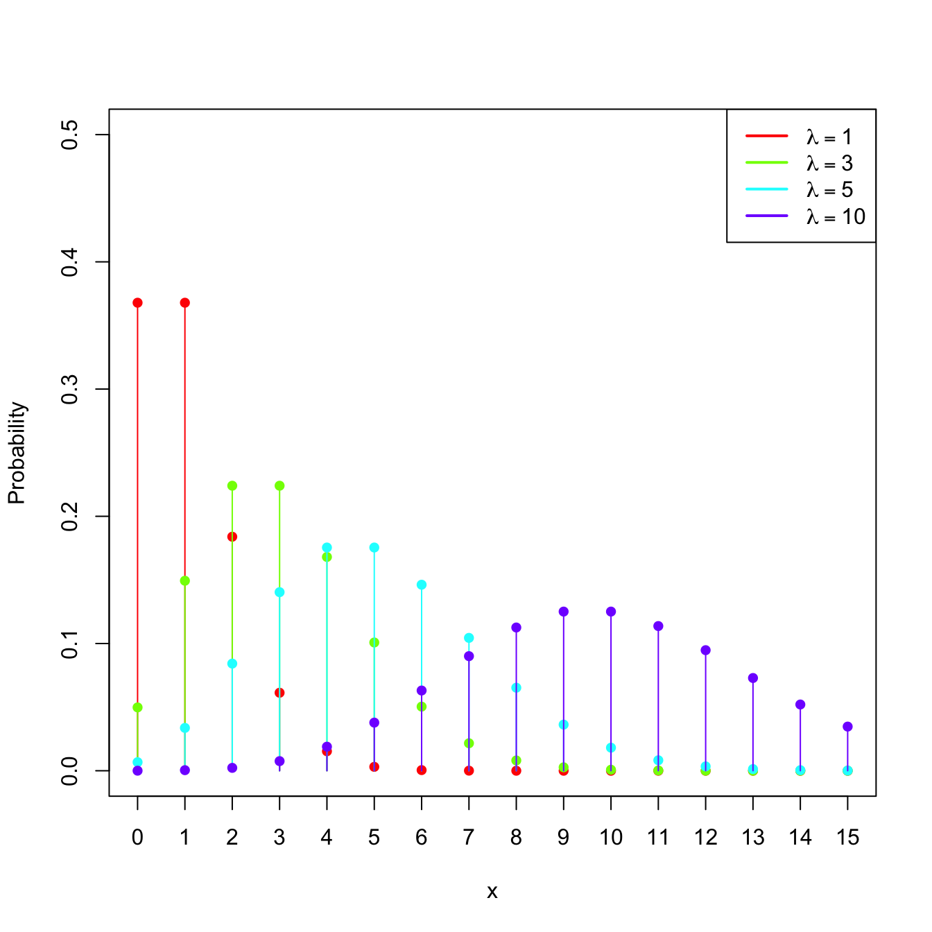
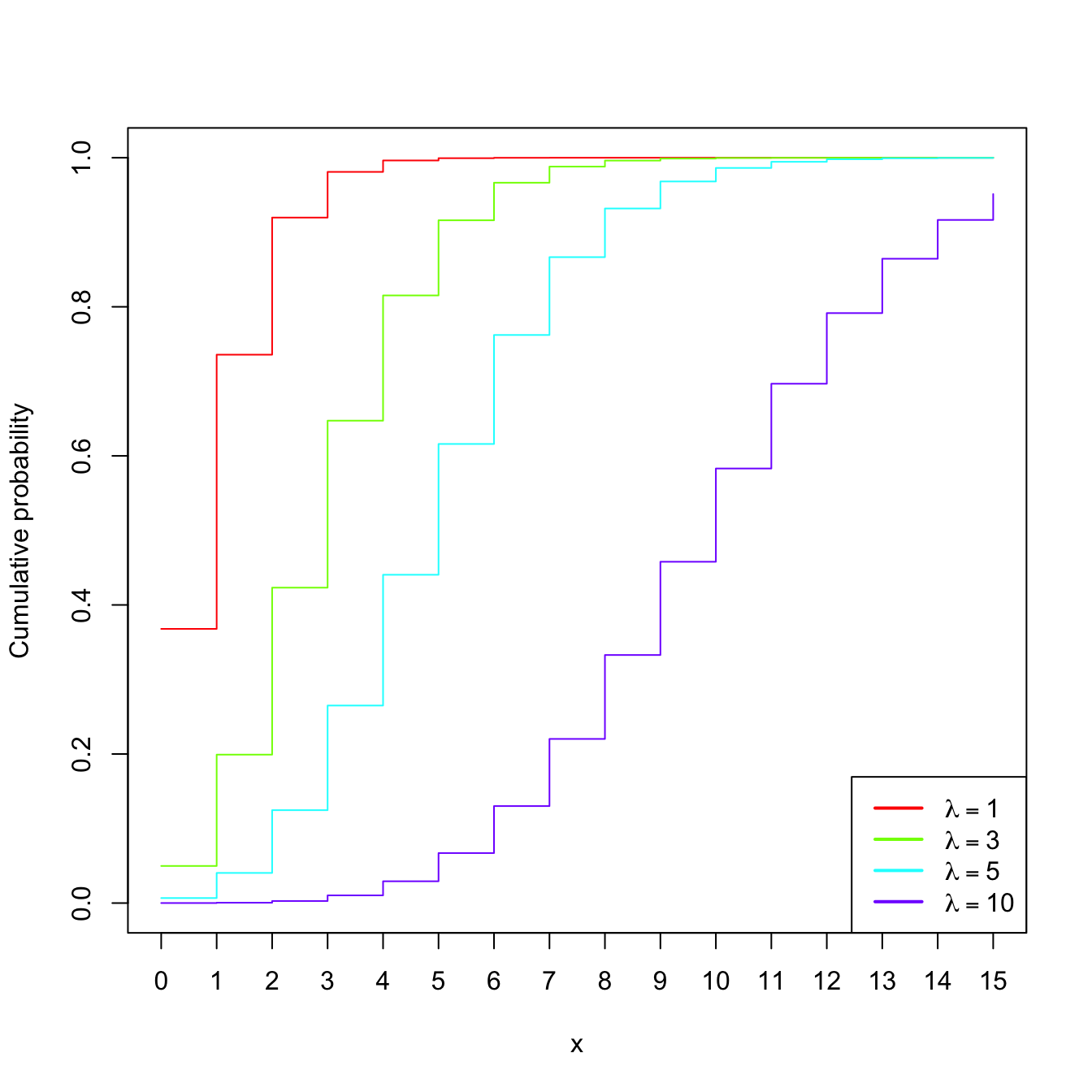
Figure 1.5: $\mathrm{Pois}(\lambda)$ pmf’s and cdf’s for several intensities $\lambda.$

Example 1.15 (Binomial model) The random variable $X\sim\mathrm{Bin}(n,p),$ with $n\in\mathbb{N}$ and $p\in[0,1],$ is such that its pmf is

$$\begin{align*} p(x;n,p)=\binom{n}{x}p^x(1-p)^{n-x},\quad x=0,1,\ldots,n. \end{align*}$$

The points $\{0,1,\ldots,n\}$ are the atoms of $X.$ This probability model is designed to sum the successes of a random experiment with probability of success $p$ that is independently repeated $n$ times.

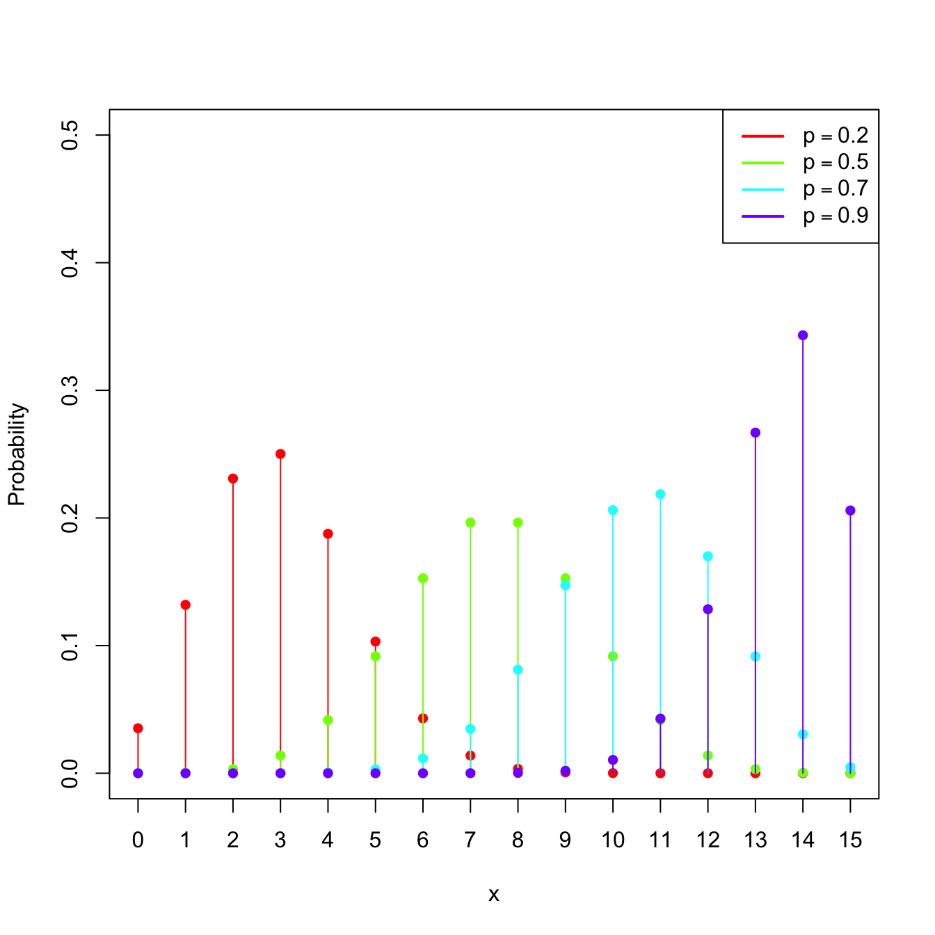
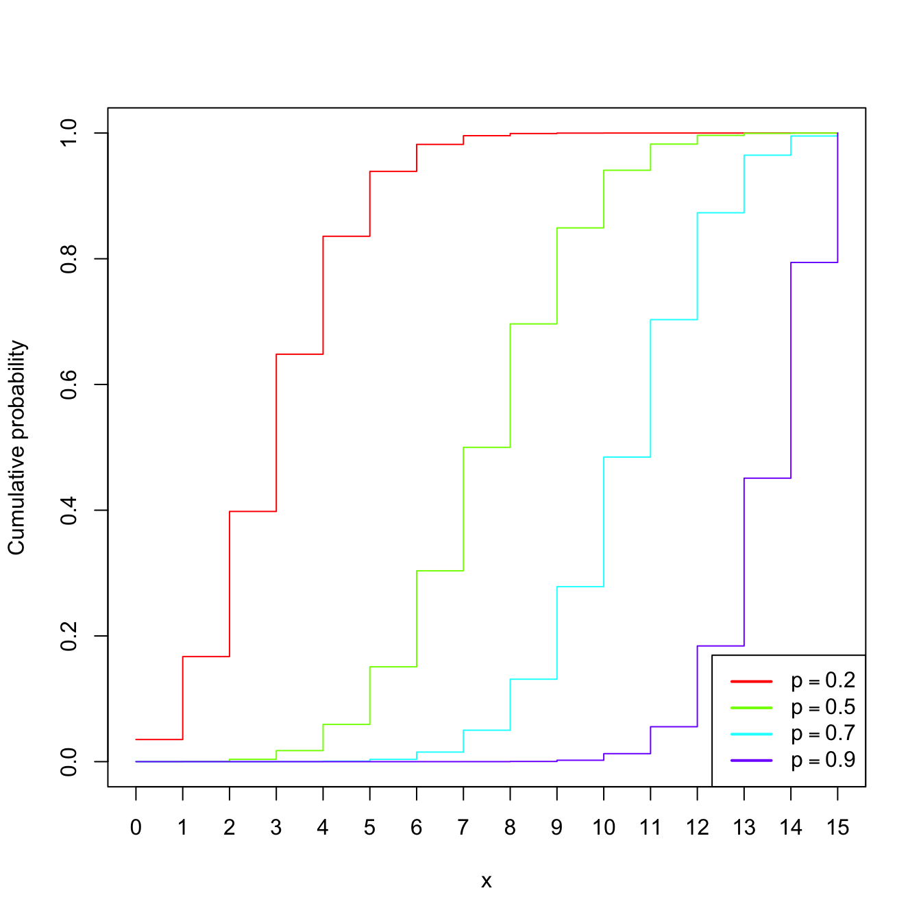
Figure 1.6: $\mathrm{Bin}(n,p)$ pmf’s and cdf’s for size $n=15$ and several probabilities $p.$

Example 1.16 (Uniform (continuous)) The random variable $X\sim\mathcal{U}(a,b),$ $a<b,$ is such that its pdf is

$$\begin{align*} f(x;a,b)=\begin{cases} 1/(b-a),& x\in(a,b),\\ 0,&\text{otherwise.} \end{cases} \end{align*}$$

Example 1.17 (Normal model) The random variable $X\sim\mathcal{N}(\mu,\sigma^2)$ (notice the second argument is a variance), with mean $\mu\in\mathbb{R}$ and standard deviation $\sigma>0,$ has pdf

$$\begin{align*} \phi(x;\mu,\sigma^2):=\frac{1}{\sqrt{2\pi}\sigma}\exp\left\{-\frac{(x-\mu)^2}{2\sigma^2}\right\},\quad x\in\mathbb{R}. \end{align*}$$

This probability model is extremely useful to model many random variables in reality, especially those that are composed of sums of other random variables (why?).

The standard normal distribution is $\mathcal{N}(0,1).$ A standard normal rv is typically denoted by $Z,$ its pdf by simply $\phi,$ and its cdf by

$$\begin{align*} \Phi(x):=\int_{-\infty}^x \phi(t)\,\mathrm{d}t. \end{align*}$$

The cdf of $\mathcal{N}(\mu,\sigma^2)$ is $\Phi\left(\frac{\cdot-\mu}{\sigma}\right).$

Example 1.18 (Exponential model) The random variable $X\sim\mathrm{Exp}(\lambda),$ $\lambda>0$ (rate parameter), has pdf

$$\begin{align*} f(x;\lambda)=\lambda e^{-\lambda x},\quad x\in\mathbb{R}_+. \end{align*}$$

This probability model is useful to model lifetimes.

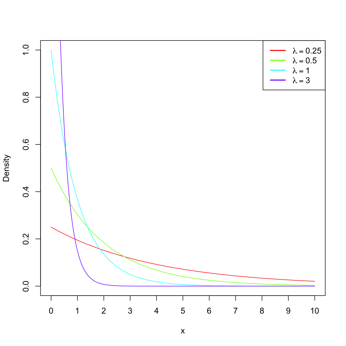
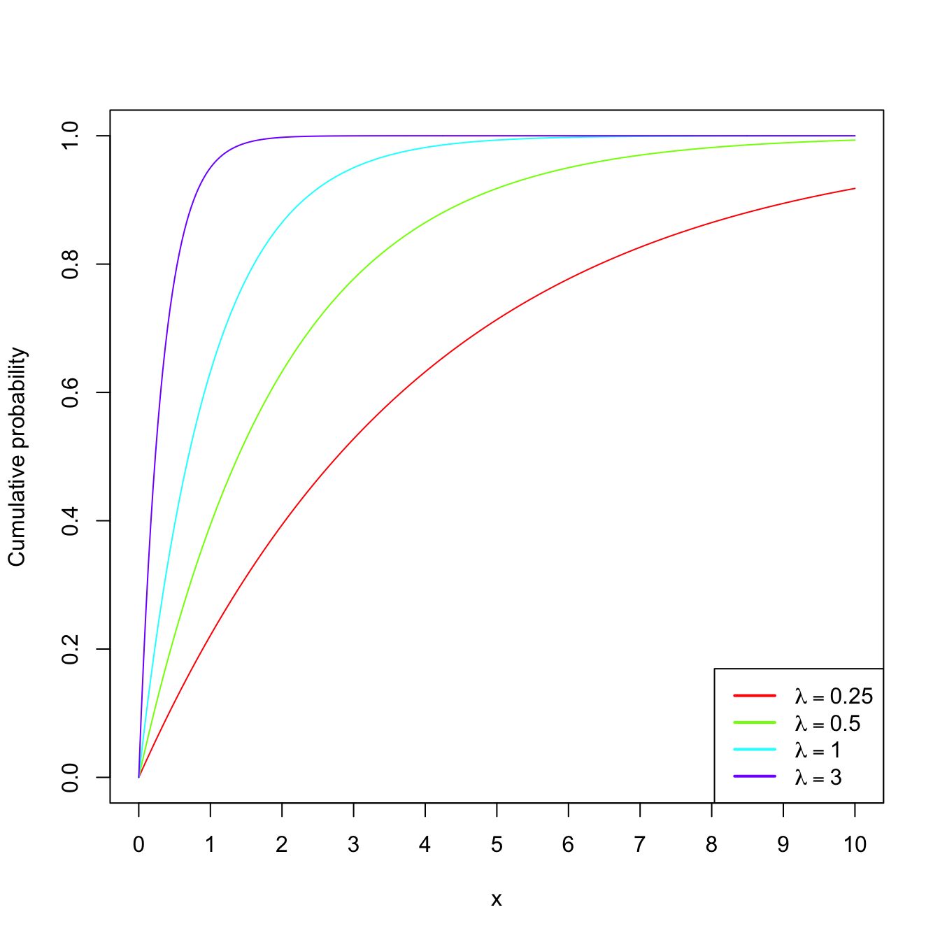
Figure 1.7: $\mathrm{Exp}(\lambda)$ pdf’s and cdf’s for several rates $\lambda.$

1.2.2 Expectation and variance

Definition 1.19 (Expectation) Given a random variable $X\sim F_X,$ its expectation $\mathbb{E}[X]$ is defined as⁸

$$\begin{align*} \mathbb{E}[X]:=&\;\int x\,\mathrm{d}F_X(x)\\ :=&\;\begin{cases} \displaystyle\int_{\mathbb{R}} x f_X(x)\,\mathrm{d}x,&\text{ if }X\text{ is continuous,}\\ \displaystyle\sum_{\{x\in\mathbb{R}:p_X(x)>0\}} xp_X(x),&\text{ if }X\text{ is discrete.} \end{cases} \end{align*}$$

Example 1.19 Let $X\sim \mathcal{U}(a,b).$ Then:

$$\begin{align*} \mathbb{E}[X]=&\;\int_{\mathbb{R}} x f(x;a,b)\,\mathrm{d}x=\frac{1}{b-a}\int_a^b x \,\mathrm{d}x\\ =&\;\frac{1}{b-a}\frac{b^2-a^2}{2}=\frac{a+b}{2}. \end{align*}$$

Definition 1.20 (Variance and standard deviation) The variance of the random variable $X$ is defined as

$$\begin{align*} \mathbb{V}\mathrm{ar}[X]:=\mathbb{E}[(X-\mathbb{E}[X])^2] =\mathbb{E}[X^2]-\mathbb{E}[X]^2. \end{align*}$$

The standard deviation of $X$ is $\sqrt{\mathbb{V}\mathrm{ar}[X]}.$

Example 1.20 Let $X\sim \mathrm{Pois}(\lambda).$ Then:

$$\begin{align*} \mathbb{E}[X]=&\;\sum_{\{x\in\mathbb{R}:p(x;\lambda)>0\}} x p(x;\lambda)=\sum_{x=0}^\infty x \frac{e^{-\lambda}\lambda^x}{x!}\\ =&\;e^{-\lambda}\sum_{x=1}^\infty \frac{\lambda^x}{(x-1)!}=e^{-\lambda} \lambda \sum_{x=0}^\infty \frac{\lambda^x}{x!}\\ =&\;\lambda \end{align*}$$

using that $e^\lambda=\sum_{x=0}^\infty \frac{\lambda^x}{x!}.$ Similarly,⁹

$$\begin{align*} \mathbb{E}[X^2]=&\;\sum_{x=0}^\infty x^2 \frac{e^{-\lambda}\lambda^x}{x!}=e^{-\lambda} \sum_{x=1}^\infty \frac{x\lambda^x}{(x-1)!}\\ =&\;e^{-\lambda} \lambda \sum_{x=0}^\infty \{1+x\}\frac{\lambda^x}{x!}=e^{-\lambda} \lambda \bigg\{e^{\lambda} + \sum_{x=1}^\infty x \frac{\lambda^x}{x!}\bigg\}\\ =&\;\lambda + e^{-\lambda} \lambda^2 \sum_{x=0}^\infty \frac{\lambda^x}{x!}=\lambda(1+\lambda). \end{align*}$$

Therefore, $\mathbb{V}\mathrm{ar}[X]=\lambda(1+\lambda)-\lambda^2=\lambda.$

A deeper and more general treatment of expectation and variance is given in Section 1.3.4.

1.2.3 Moment generating function

Definition 1.21 (Moment generating function) The moment generating function (mgf) of a rv $X$ is the function

$$\begin{align*} M_X(s):=\mathbb{E}\left[e^{sX}\right], \end{align*}$$

for $s\in(-h,h)\subset \mathbb{R},$ $h>0,$ and such that the expectation $\mathbb{E}\left[e^{sX}\right]$ exists. If the expectation does not exist for any neighborhood around zero, then we say that the mgf does not exist.¹⁰

Remark. In analytical terms, the mgf for a continuous random variable $X$ is the bilateral Laplace transform of the pdf $f_X$: $F(s):= \int_{-\infty}^{\infty}e^{-st}f_X(t)\,\mathrm{d}t.$ If $X>0,$ then the mgf is simply the Laplace transform of $f_X$: $\mathcal{L}\{f\}(s):= \int_{0}^{\infty}e^{-st}f_X(t)\,\mathrm{d}t.$

Example 1.21 (Gamma mgf) A rv $X$ follows a gamma distribution with shape $\alpha$ and scale $\beta,$ denoted as $X\sim\Gamma(\alpha,\beta),$ if its pdf belongs to the next parametric class of densities:

$$\begin{align*} f(x;\alpha,\beta)=\frac{1}{\Gamma(\alpha)\beta^{\alpha}}x^{\alpha-1}e^{-x/\beta}, \quad x>0, \ \alpha>0,\ \beta>0, \end{align*}$$

where $\Gamma(\alpha)$ is the gamma function, defined as

$$\begin{align*} \Gamma(\alpha):=\int_{0}^{\infty} x^{\alpha-1}e^{-x}\,\mathrm{d}x. \end{align*}$$

The gamma function satisfies the following properties:

• $\Gamma(1)=1.$
• $\Gamma(\alpha)=(\alpha-1)\Gamma(\alpha-1),$ for any $\alpha\geq 1.$
• $\Gamma(n)=(n-1)!,$ for any $n\in\mathbb{N}.$

Let us compute the mgf of $X$:

$$\begin{align*} M_X(s)&=\mathbb{E}\left[e^{sX}\right]\\ &=\frac{1}{\Gamma(\alpha)\beta^{\alpha}}\int_{0}^{\infty} e^{sx} x^{\alpha-1}e^{-x/\beta}\,\mathrm{d}x\\ &=\frac{1}{\Gamma(\alpha)\beta^{\alpha}}\int_{0}^{\infty} x^{\alpha-1}e^{-(1/\beta -s)x}\,\mathrm{d}x\\ &=\frac{1}{\Gamma(\alpha)\beta^{\alpha}}\int_{0}^{\infty} x^{\alpha-1}e^{-x/(1/\beta -s)^{-1}}\,\mathrm{d}x. \end{align*}$$

The kernel of a pdf is the main part of the density once the constants are removed. Observe that in the integrand we have the kernel of a gamma pdf with shape $\alpha$ and scale $(1/\beta-s)^{-1}=\beta/(1-s\beta).$ If $s\geq 1/\beta,$ then the integral is $\infty.$ However, if $s<1/\beta,$ then the integral is finite, and multiplying and dividing by the adequate constants, we obtain the mgf

$$\begin{align*} M_X(s)&=\frac{1}{\beta^{\alpha}}\left(\frac{\beta}{1-s\beta}\right)^{\alpha} \int_{0}^{\infty} \frac{1}{\Gamma(\alpha)}\left(\frac{\beta}{1-s\beta}\right)^{-\alpha} x^{\alpha-1}e^{-\frac{x}{\beta/(1-s\beta)}} \,\mathrm{d}x\\ &=\frac{1}{(1-s\beta)^{\alpha}}, \quad s<1/\beta. \end{align*}$$

Recall that, since $\beta>0,$ the mgf exists in the interval $(-h,h)$ with $h=1/\beta;$ see Figure 1.8 for graphical insight.

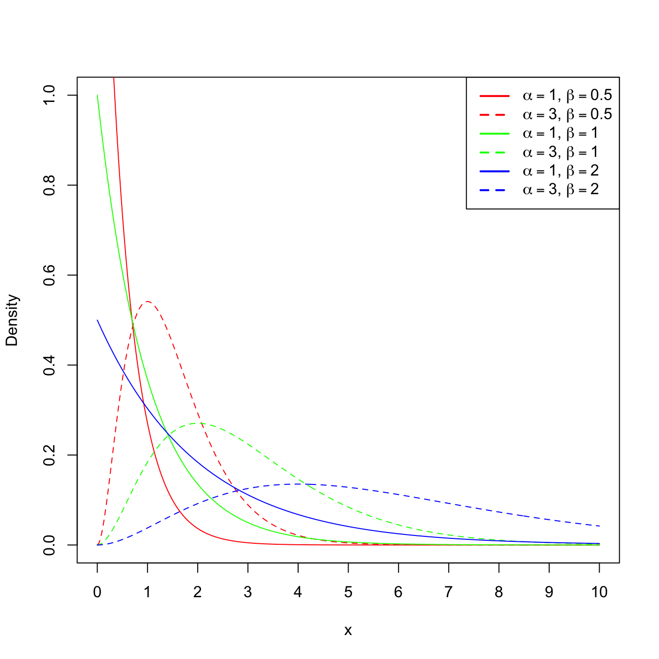
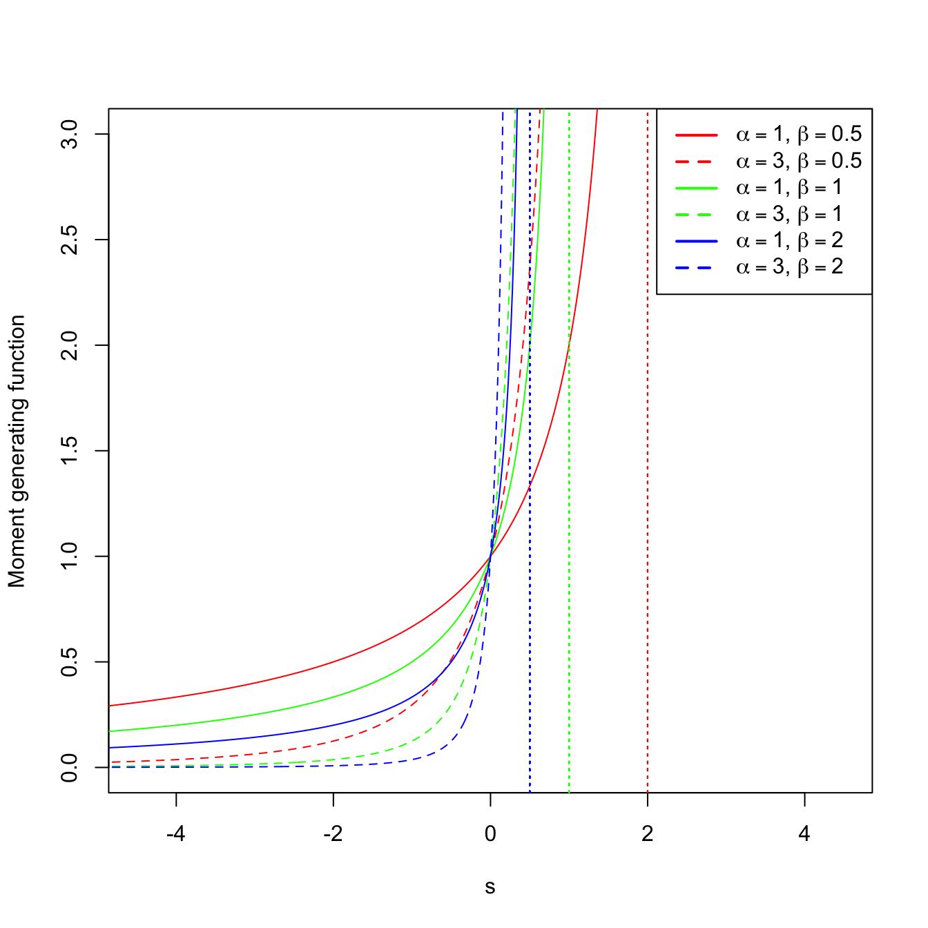
Figure 1.8: $\Gamma(\alpha,\beta)$ pdf’s and mgf’s for several shapes $\alpha$ and scales $\beta.$ The dotted vertical lines represent the value $s=1/\beta.$

Example 1.22 (Binomial mgf) As seen in Example 1.15, the pmf of $\mathrm{Bin}(n,p)$ is

$$\begin{align*} p(x;n,p)=\binom{n}{x} p^x (1-p)^{n-x}, \quad x=0,1,2,\ldots \end{align*}$$

Let us compute its mgf:

$$\begin{align*} M_X(s)=\sum_{x=0}^{\infty} e^{sx}\binom{n}{x} p^x (1-p)^{n-x}=\sum_{x=0}^{\infty} \binom{n}{x} (pe^s)^x (1-p)^{n-x}. \end{align*}$$

By Newton’s generalized binomial theorem, we know that¹¹

$$\begin{align} (a+b)^r =\sum_{x=0}^{\infty} \binom{r}{x} a^x b^{r-x},\quad a,b,r\in\mathbb{R},\tag{1.3} \end{align}$$

and therefore the mgf is

$$\begin{align*} M_X(s)=(pe^s+1-p)^n, \quad \forall s\in\mathbb{R}. \end{align*}$$

The mgf is shown in Figure 1.9, which displays how $M_X$ is continuous despite the pmf being discrete.

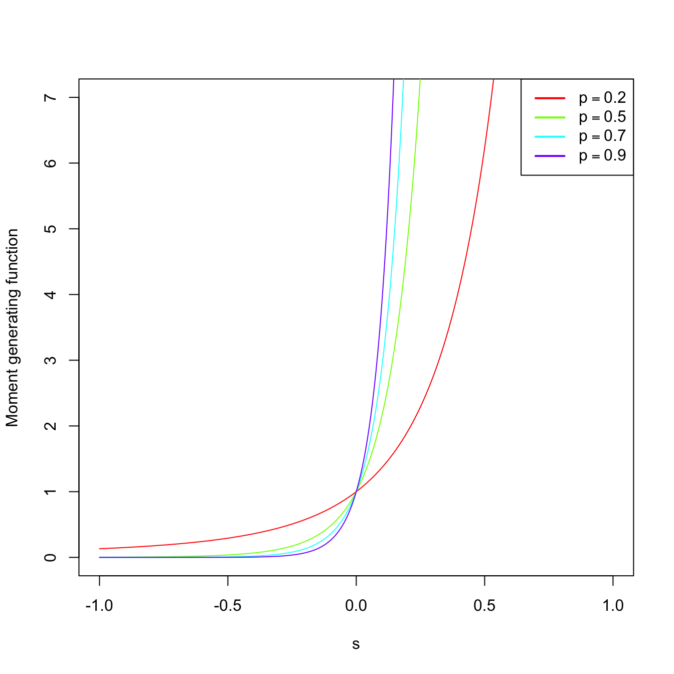
Figure 1.9: $\mathrm{Bin}(n,p)$ pmf’s and mgf’s for size $n=15$ and several probabilities $p.$

The following theorem says that, as its name indicates, the mgf of a rv $X$ indeed generates the raw moments of $X$ (that is, the moments centered about $0$).

Theorem 1.1 (Moment generation by the mgf) Let $X$ be a rv with mgf $M_X.$ Then,

$$\begin{align*} \mathbb{E}[X^n]=M_X^{(n)}(0), \end{align*}$$

where $M_X^{(n)}(0)$ denotes the $n$-th derivative of the mgf with respect to $s,$ evaluated at $s=0.$

Example 1.23 Let us compute the expectation and variance of $X\sim\Gamma(\alpha,\beta).$ Using Theorem 1.1 and Example 1.21,

$$\begin{align*} \mathbb{E}[X]=M_X^{(1)}(0)=\left.\frac{\mathrm{d}}{\mathrm{d} s}\frac{1}{(1-s\beta)^{\alpha}}\right\vert_{s=0}=\left.\frac{\alpha\beta}{(1-s\beta)^{\alpha+1}}\right\vert_{s=0}=\alpha\beta. \end{align*}$$

Analogously,

$$\begin{align*} \mathbb{E}[X^2]=M_X^{(2)}(0)=\left.\frac{\mathrm{d}^2}{\mathrm{d} s^2}\frac{1}{(1-s\beta)^{\alpha}}\right\vert_{s=0}=\left. \frac{\alpha(\alpha+1)\beta^2}{(1-s\beta)^{\alpha+2}}\right\vert_{s=0}=\alpha(\alpha+1)\beta^2. \end{align*}$$

Therefore,

$$\begin{align*} \mathbb{V}\mathrm{ar}[X]=\mathbb{E}[X^2]-\mathbb{E}[X]^2=\alpha(\alpha+1)\beta^2-\alpha^2\beta^2=\alpha\beta^2. \end{align*}$$

The result below is important because it shows that the distribution of a rv is determined from its mgf.

Theorem 1.2 (Uniqueness of the mgf) Let $X$ and $Y$ two rv’s with mgf’s $M_X$ and $M_Y,$ respectively. If

$$\begin{align*} M_X(s)=M_Y(s), \quad \forall s\in (-h,h), \end{align*}$$

then the distributions of $X$ and $Y$ are the same.

The following properties of the mgf are very useful to manipulate mgf’s of linear combinations of independent random variables.

Proposition 1.5 (Properties of the mgf) The mgf satisfies the following properties:

1. Let $X$ be a rv with mgf $M_X.$ Define the rv $$\begin{align*} Y=aX+b, \quad a,b\in \mathbb{R}, \ a\neq 0. \end{align*}$$ Then, the mgf of the new rv $Y$ is $$\begin{align*} M_Y(s)=e^{sb}M_X(as). \end{align*}$$

2. Let $X_1,\ldots,X_n$ be independent¹² rv’s with mgf’s $M_{X_1},\ldots,M_{X_n},$ respectively. Let be the rv $$\begin{align*} Y=X_1+\cdots+X_n. \end{align*}$$ Then, its mgf is given by $$\begin{align*} M_Y(s)=\prod_{i=1}^n M_{X_i}(s). \end{align*}$$

Proof (Proof of Proposition 1.5). In order to see i, observe that

$$\begin{align*} M_Y(s)&=\mathbb{E}\left[e^{sY}\right]=\mathbb{E}\left[e^{s(aX+b)}\right]=\mathbb{E}\left[e^{saX}e^{sb}\right]\\ &=e^{sb}\mathbb{E}\left[e^{saX}\right]=e^{sb}M_X(as). \end{align*}$$

To check ii, consider

$$\begin{align*} M_Y(s)&=\mathbb{E}\left[e^{sY}\right]=\mathbb{E}\left[e^{s\sum_{i=1}^n X_i}\right]=\mathbb{E}\left[e^{sX_1}\cdots e^{sX_n}\right]\\ &=\mathbb{E}\left[e^{sX_1}\right]\cdots \mathbb{E}\left[e^{sX_n}\right]=\prod_{i=1}^n M_{X_i}(s). \end{align*}$$

The equality $\mathbb{E}\left[e^{sX_1}\cdots e^{sX_n}\right]=\mathbb{E}\left[e^{sX_1}\right]\cdots \mathbb{E}\left[e^{sX_n}\right]$ is only satisfied because of the independence of $X_1,\ldots,X_n.$

The next theorem is very useful for proving convergence in distribution¹³ of random variables by employing a simple-to-use function such as the mgf. For example, the central limit theorem, a cornerstone result in statistical inference, can be easily proved using Theorem 1.3.

Theorem 1.3 (Convergence of the mgf) Assume that $X_n,$ $n=1,2,\ldots$ is a sequence of rv’s with respective mgf’s $M_{X_n},$ $n\geq 1.$ Assume in addition that, for all $s\in(-h,h)$ with $h>0,$ it holds

$$\begin{align*} \lim_{n\to\infty} M_{X_n}(s)=M_X(s), \end{align*}$$

where $M_X$ is a mgf. Then there exists a unique cdf $F_X$ whose moments are determined by $M_X$ and, for all $x$ where $F_X(x)$ is continuous, it holds

$$\begin{align*} \lim_{n\to\infty} F_{X_n}(x)=F_X(x). \end{align*}$$

That is, the convergence of mgf’s implies the convergence of cdf’s.

---

3. The following is an analogy with the hierarchy in computer languages: $(\mathbb{R},\mathcal{B})$ is the high-level programming language, $X$ is the compiler, and $(\Omega,\mathcal{A})$ is the low-level programming language that is run by the machine.↩︎

4. That is, $\lim_{x\to a+} F_X(x)=F(a),$ for all $a\in\mathbb{R}.$↩︎

5. This terminology stems from the fact that the existence of $f_X$ such that condition (1.2) holds is equivalent to $F_X$ being an absolutely continuous function. As the famous counterexample given by the Cantor function, absolute continuity is a more strict requirement than continuity.↩︎

6. “Almost all” meaning that a finite or countable number of points is excluded.↩︎

7. Observe $\int_{(a,b)} f_X(t)\,\mathrm{d}t=\int_a^b f_X(t)\,\mathrm{d}t.$↩︎

8. “$\mathrm{d}F_X(x)$” is just a fancy way of combining the continuous case (integral) and discrete case (sum) within the same notation. The precise mathematical meaning of “$\mathrm{d}F_X(x)$” is the Riemann–Stieltjes integral.↩︎

9. See the forthcoming “Law of the unconscious statistician” in Proposition 1.10.↩︎

10. The possible non-existence can be removed considering the characteristic function $\varphi_X(t)=\mathbb{E}\left[e^{\mathrm{i}tX}\right],$ which exists for all $t\in\mathbb{R}.$ However, it comes at the expense of having a complex-valued function ($\mathrm{i}=\sqrt{-1}$ is the imaginary unit). The properties of the mgf and characteristic function are almost equivalent since $\varphi_X(-\mathrm{i}t)=M_X(t).$↩︎

11. Observe if $r$ in (1.3) is a natural number, then the standard binomial theorem arises since $\binom{r}{x}=0$ when $x>r$: $(a+b)^r =\sum_{x=0}^{r} \binom{r}{x} a^x b^{r-x}.$↩︎

12. A formal definition of independence of rv’s is given in the forthcoming Definition 1.34.↩︎

13. This concept will be precised in the forthcoming Definition 2.6.↩︎