6.6 Power of a test and Neyman–Pearson’s Lemma

Definition 6.6 (Power function) The power function of a test $\varphi$ is the function $\omega:\Theta\rightarrow[0,1]$ that gives the probability of rejecting $H_0$ from a srs $(X_1,\ldots,X_n)$ generated from $F(\cdot;\theta),$ for each $\theta\in\Theta$:

\[\begin{align*} \omega(\theta)=\mathbb{P}(\text{Reject $H_0$}|\theta)=\mathbb{P}(\varphi(X_1,\ldots,X_n)=1|\theta). \end{align*}\]

Remark. Recall that for $\theta=\theta_0\in\Theta_0$ and $H_0:\theta=\theta_0,$ the power equals the significance level:

\[\begin{align*} \omega(\theta_0)=\mathbb{P}(\text{Reject $H_0$}|\theta_0)=\alpha. \end{align*}\]

In addition, for any value $\theta=\theta_1\in\Theta_1,$

\[\begin{align*} \omega(\theta_1)=\mathbb{P}(\text{Reject $H_0$}|\theta_1)=1-\mathbb{P}(\text{Do not reject $H_0$}|\theta_1)=1-\beta(\theta_1), \end{align*}\]

that is, the power in $\theta_1$ equals the complementary of the Type II error probability for $\theta_1$ seen in Section 6.1.

Remark. Observe that the power function of the test $\varphi$ is only informative on the expected behavior of $\varphi;$ the function does not depend on the particular sample realization at hand.

Example 6.18 Consider $(X_1,\ldots,X_n)$ a srs of $\mathcal{N}(\mu,\sigma^2)$ with $\sigma^2$ known, the test statistic

\[\begin{align*} T(X_1,\ldots,X_n)=\frac{\bar{X}-\mu_0}{\sigma/\sqrt{n}} \end{align*}\]

and the hypothesis tests

$H_0:\mu=\mu_0$ vs. $H_1:\mu>\mu_0;$
$H_0:\mu=\mu_0$ vs. $H_1:\mu<\mu_0;$
$H_0:\mu=\mu_0$ vs. $H_1:\mu\neq\mu_0$

with rejection regions

$C_a=\{Z>z_{\alpha}\};$
$C_b=\{Z<-z_{\alpha}\};$
$C_c=\{|Z|>z_{\alpha/2}\}.$

Let us compute and plot the power functions for the testing problems a, b, and c.

In the first case:

\[\begin{align*} \omega_a(\mu)&=\mathbb{P}(T(X_1,\ldots,X_n)>z_{\alpha})=\mathbb{P}\left(\frac{\bar{X}-\mu_0}{\sigma/\sqrt{n}}>z_{\alpha}\right)\\ &=\mathbb{P}\left(\frac{\bar{X}-\mu_0+(\mu-\mu)}{\sigma/\sqrt{n}}>z_{\alpha}\right)=\mathbb{P}\left(\frac{\bar{X}-\mu}{\sigma/\sqrt{n}}>z_{\alpha}-\frac{\mu-\mu_0}{\sigma/\sqrt{n}}\right)\\ &=\mathbb{P}\left(-Z<-z_{\alpha}+\frac{\mu-\mu_0}{\sigma/\sqrt{n}}\right)=\mathbb{P}\left(Z<-z_{\alpha}+\frac{\mu-\mu_0}{\sigma/\sqrt{n}}\right)\\ &=\Phi\left(-z_{\alpha}+\frac{\mu-\mu_0}{\sigma/\sqrt{n}}\right), \end{align*}\]

where $Z\sim\mathcal{N}(0,1).$ As expected, $\omega_a(\mu_0)=\Phi(-z_{\alpha})=\alpha.$

The second case is analogous:

\[\begin{align*} \omega_b(\mu)&=\mathbb{P}(T(X_1,\ldots,X_n)<-z_{\alpha})=\mathbb{P}\left(Z<-z_{\alpha}-\frac{\mu-\mu_0}{\sigma/\sqrt{n}}\right)\\ &=\Phi\left(-z_{\alpha}+\frac{\mu_0-\mu}{\sigma/\sqrt{n}}\right). \end{align*}\]

The third case follows now as a combination of the previous two ones:

\[\begin{align*} \omega_c(\mu)&=\mathbb{P}(|T(X_1,\ldots,X_n)|>z_{\alpha/2})\\ &=\mathbb{P}(T(X_1,\ldots,X_n)<-z_{\alpha/2})+\mathbb{P}(T(X_1,\ldots,X_n)>z_{\alpha/2})\\ &=\Phi\left(-z_{\alpha/2}+\frac{\mu_0-\mu}{\sigma/\sqrt{n}}\right)+\Phi\left(-z_{\alpha/2}+\frac{\mu-\mu_0}{\sigma/\sqrt{n}}\right). \end{align*}\]

For fixed $\mu_0=0,$ $\alpha=0.10,$ $n=25,$ and $\sigma=1$ we can visualize the power functions $\mu\mapsto\omega_a(\mu),$ $\mu\mapsto\omega_b(\mu),$ and $\mu\mapsto\omega_c(\mu)$ in Figure 6.2. The curves give the probability of rejection of $H_0:\mu=\mu_0$ in favor of $H_1$ using a sample of size $n,$ as a function on what is the underlying truth $\mu.$

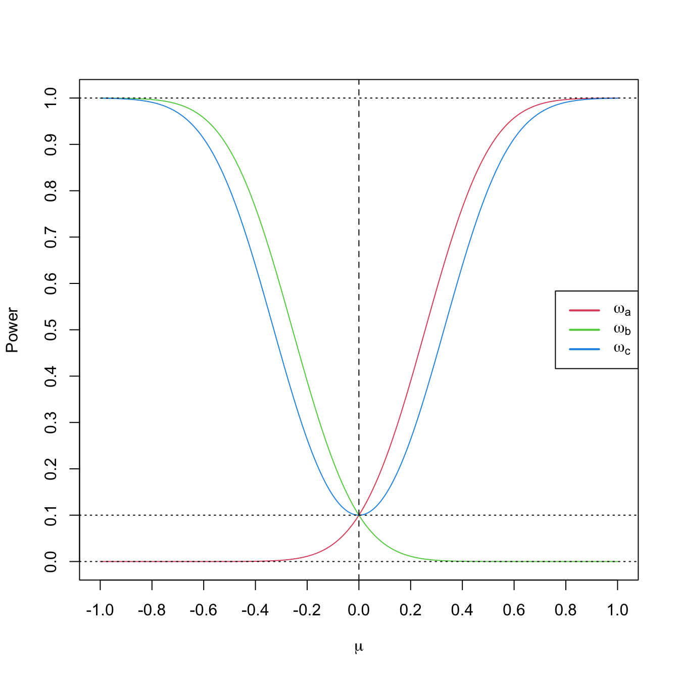
$Power functions $\mu\mapsto\omega_a(\mu),$ $\mu\mapsto\omega_b(\mu),$ and $\mu\mapsto\omega_c(\mu)$ from Example 6.18 with $\mu_0=0$ (dashed vertical line), $\alpha=0.10$ (dotted horizontal line), $n=25,$ and $\sigma=1.$ Observe how a one-sided test has power below $\alpha$ against alternatives in the opposite direction and how the two-sided test almost merges the powers of the two one-sided tests.$

Figure 6.2: Power functions $\mu\mapsto\omega_a(\mu),$ $\mu\mapsto\omega_b(\mu),$ and $\mu\mapsto\omega_c(\mu)$ from Example 6.18 with $\mu_0=0$ (dashed vertical line), $\alpha=0.10$ (dotted horizontal line), $n=25,$ and $\sigma=1.$ Observe how a one-sided test has power below $\alpha$ against alternatives in the opposite direction and how the two-sided test almost merges the powers of the two one-sided tests.

The usual criterion for selecting among several types of tests for the same hypothesis consists in fixing the Type I error probability, $\alpha,$ and then selecting among the tests with the same Type I error the one that presents the highest power for all $\theta_1\in\Theta_1.$ This is the so-called Uniformly Most Powerful (UMP) test. However, the UMP test does not always exists.

The Neyman–Pearson’s Lemma guarantees the existence of the UMP test for the testing problem in which the null and the alternative hypotheses are simple, and provides us the form of the critical region for such a test. This region is based on a ratio of the likelihoods of the two parameter values appearing in $H_0$ and $H_1.$

Theorem 6.1 (Neyman–Pearson’s Lemma) Let $X\sim F(\cdot;\theta).$ Assume it is desired to test

\[\begin{align} H_0:\theta=\theta_0\quad \text{vs.}\quad H_1:\theta=\theta_1 \tag{6.5} \end{align}\]

using the information of a srs $(X_1,\ldots,X_n)$ of $X.$ For the significance level $\alpha,$ the test that maximizes the power in $\theta_1$ has a critical region of the form

\[\begin{align*} C=\left\{(x_1,\ldots,x_n)'\in\mathbb{R}^n:\frac{\mathcal{L}(\theta_0;x_1,\ldots,x_n)}{\mathcal{L}(\theta_1;x_1,\ldots,x_n)}<k\right\}. \end{align*}\]

Recall that the Neyman–Pearson’s Lemma specifies only the form of the critical region, but not the specific value of $k.$ However, $k$ could be computed from the significance level $\alpha$ and the distribution of $(X_1,\ldots,X_n)$ under $H_0.$

Example 6.19 Assume that $X$ represents a single observation of the rv with pdf

\[\begin{align*} f(x;\theta)=\begin{cases} \theta x^{\theta-1}, & 0<x<1,\\ 0, & \text{otherwise}. \end{cases} \end{align*}\]

Find the UMP test at a significance level $\alpha=0.05$ for testing

\[\begin{align*} H_0: \theta=1\quad \text{vs.} \quad H_1:\theta=2. \end{align*}\]

Let us employ Theorem 6.1. In this case we have a srs of size one. Then, the likelihood is

\[\begin{align*} \mathcal{L}(\theta;x)=\theta x^{\theta-1}. \end{align*}\]

For computing the critical region of the UMP test, we obtain

\[\begin{align*} \frac{\mathcal{L}(\theta_0;x)}{\mathcal{L}(\theta_1;x)}=\frac{\mathcal{L}(1;x)}{\mathcal{L}(2;x)}=\frac{1}{2x} \end{align*}\]

and therefore

\[\begin{align*} C=\left\{x\in\mathbb{R}:\frac{1}{2x}<k\right\}=\left\{x>\frac{1}{2k}\right\}=\{x>k'\}. \end{align*}\]

The value of $k'$ can be determined from the significance level $\alpha,$

\[\begin{align*} \alpha&=\mathbb{P}(\text{Reject $H_0$}|\text{$H_0$ true})=\mathbb{P}(x>k'|\theta=1)\\ &=\int_{k'}^1 f(x;1)\,\mathrm{d}x=\int_{k'}^{1}\,\mathrm{d}x=1-k'. \end{align*}\]

Therefore, $k'=1-\alpha,$ so the critical region of UMP test of size $\alpha$ is

\[\begin{align*} C=\{x:x>1-\alpha\}. \end{align*}\]

When testing one-sided hypothesis of the type

\[\begin{align} H_0:\theta=\theta_0\quad \text{vs.}\quad H_1:\theta>\theta_0,\tag{6.6} \end{align}\]

the Neyman–Pearson’s Lemma is not applicable.

However, if we fix a value $\theta_1>\theta_0$ and we compute the critical region of the UMP test for

\[\begin{align*} H_0:\theta=\theta_0\quad \text{vs.}\quad H_1:\theta=\theta_1, \end{align*}\]

quite often the critical region obtained does not depend on the value $\theta_1.$ Therefore, this very same test is the UMP test for testing (6.6)!

In addition, if we have an UMP test for

\[\begin{align*} H_0:\theta=\theta_0\quad \text{vs.}\quad H_1:\theta>\theta_0, \end{align*}\]

then the same test is also the UMP test for

\[\begin{align*} H_0:\theta=\theta_0'\quad \text{vs.}\quad H_1:\theta>\theta_0, \end{align*}\]

since for any value $\theta_0'<\theta_0,$ any other test will have larger errors of the two types.