5.3 Confidence intervals on two normal populations

We assume now that we have two independent populations $X_1\sim \mathcal{N}(\mu_1,\sigma_1^2)$ and $X_2\sim \mathcal{N}(\mu_2,\sigma_2^2)$ from which two respective srs’s $(X_{11},\ldots,X_{1n_1})$ and $(X_{21},\ldots,X_{2n_2})$ of sizes $n_1$ and $n_2$ are extracted. As in Section 5.2, the confidence intervals derived in this section arise from the sampling distributions obtained in Section 2.2 for normal populations.

5.3.1 Confidence interval for the difference of means with known variances

Assume that the mean populations $\mu_1$ and $\mu_2$ are unknown and the variances $\sigma_1^2$ and $\sigma_2^2$ are known. We wish to construct a confidence interval for the difference $\theta=\mu_1-\mu_2.$

For that, we consider an estimator of $\theta.$ An unbiased estimator is

\[\begin{align*} \hat{\theta}=\bar{X}_1-\bar{X}_2. \end{align*}\]

Since $\hat{\theta}$ is a linear combination of normal rv’s, then it is normally distributed. Its mean is easily computed as

\[\begin{align*} \mathbb{E}\big[\hat{\theta}\big]=\mathbb{E}[\bar{X}_1]-\mathbb{E}[\bar{X}_2]=\mu_1-\mu_2. \end{align*}\]

Thanks to the independence between $X_1$ and $X_2,$ the variance is⁶⁸

\[\begin{align*} \mathbb{V}\mathrm{ar}\big[\hat{\theta}\big]=\mathbb{V}\mathrm{ar}[\bar{X}_1]+\mathbb{V}\mathrm{ar}[\bar{X}_2]=\frac{\sigma_1^2}{n_1}+\frac{\sigma_2^2}{n_2}. \end{align*}\]

Then, a possible pivot is

\[\begin{align*} Z:=\frac{\bar{X}_1-\bar{X}_2-(\mu_1-\mu_2)}{\sqrt{\frac{\sigma_1^2}{n_1}+\frac{\sigma_2^2}{n_2}}}\sim\mathcal{N}(0,1). \end{align*}\]

Again, if we split evenly the significance level $\alpha$ between the two tails, then we look for constants $c_1$ and $c_2$ such that

\[\begin{align*} \mathbb{P}(c_1\leq Z\leq c_2)=1-\alpha, \end{align*}\]

that is, $c_1=-z_{\alpha/2}$ and $c_2=z_{\alpha/2}.$ Solving for $\mu_1-\mu_2,$ we obtain

\[\begin{align*} 1-\alpha &=\mathbb{P}\left(-z_{\alpha/2}\leq \frac{\bar{X}_1-\bar{X}_2-(\mu_1-\mu_2)}{\sqrt{\frac{\sigma_1^2}{n_1}+\frac{\sigma_2^2}{n_2}}}\leq z_{\alpha/2}\right) \\ &=\mathbb{P}\left(-z_{\alpha/2}\sqrt{\frac{\sigma_1^2}{n_1}+\frac{\sigma_2^2}{n_2}}\leq \bar{X}_1-\bar{X}_2-(\mu_1-\mu_2)\leq z_{\alpha/2}\sqrt{\frac{\sigma_1^2}{n_1}+\frac{\sigma_2^2}{n_2}}\right)\\ &=\mathbb{P}\left(-(\bar{X}_1-\bar{X}_2)-z_{\alpha/2}\sqrt{\frac{\sigma_1^2}{n_1}+\frac{\sigma_2^2}{n_2}}\leq -(\mu_1-\mu_2)\leq -(\bar{X}_1-\bar{X}_2)+z_{\alpha/2}\sqrt{\frac{\sigma_1^2}{n_1}+\frac{\sigma_2^2}{n_2}}\right)\\ &=\mathbb{P}\left(\bar{X}_1-\bar{X}_2-z_{\alpha/2}\sqrt{\frac{\sigma_1^2}{n_1}+\frac{\sigma_2^2}{n_2}}\leq \mu_1-\mu_2\leq \bar{X}_1-\bar{X}_2+z_{\alpha/2}\sqrt{\frac{\sigma_1^2}{n_1}+\frac{\sigma_2^2}{n_2}}\right). \end{align*}\]

Therefore, a confidence interval for $\mu_1-\mu_2$ at the confidence level $1-\alpha$ is

\[\begin{align*} \mathrm{CI}_{1-\alpha}(\mu_1-\mu_2)=\left[\bar{X}_1-\bar{X}_2 \mp z_{\alpha/2}\sqrt{\frac{\sigma_1^2}{n_1}+\frac{\sigma_2^2}{n_2}}\right]. \end{align*}\]

Example 5.5 A new training method for an assembly operation is being tested at a factory. For that purpose, two groups of nine employees were trained during three weeks. One group was trained with the usual procedure and the other with the new method. The assembly time (in minutes) that each employee required after the training period is collected in the table below. Assuming that the assembly times are normally distributed with both variances equal to $22$ minutes, obtain a confidence interval at significance level $0.05$ for the difference of average assembly times for the two kinds of training.

Procedure	Measurements
Standard	$32 \qquad 37 \qquad 35 \qquad 28 \qquad 41 \qquad 44 \qquad 35 \qquad 31 \qquad 34$
New	$35 \qquad 31 \qquad 29 \qquad 25 \qquad 34 \qquad 40 \qquad 27 \qquad 32 \qquad 31$

The average assembly times of the two groups are

\[\begin{align*} \bar{X}_1\approx35.22,\quad \bar{X}_2\approx31.56. \end{align*}\]

Then, a confidence interval for $\mu_1-\mu_2$ at the $0.95$ confidence level is

\[\begin{align*} \mathrm{CI}_{0.95}(\mu_1-\mu_2)&\approx\left[(35.22-31.56)\mp 1.96\times 4.69\sqrt{1/9+1/9}\right]\\ &\approx[3.66\mp 4.33]=[-0.67,7.99]. \end{align*}\]

In R:

# Samples
X_1 <- c(32, 37, 35, 28, 41, 44, 35, 31, 34)
X_2 <- c(35, 31, 29, 25, 34, 40, 27, 32, 31)

# n1, n2, Xbar1, Xbar2, sigma2_1, sigma2_2, alpha, z_{alpha/2}
n_1 <- length(X_1)
n_2 <- length(X_2)
X_bar_1 <- mean(X_1)
X_bar_2 <- mean(X_2)
sigma2_1 <- sigma2_2 <- 22
alpha <- 0.05
z <- qnorm(alpha / 2, lower.tail = FALSE)

# CI
(X_bar_1 - X_bar_2) + c(-1, 1) * z * sqrt(sigma2_1 / n_1 + sigma2_2 / n_2)
## [1] -0.6669768  8.0003101

5.3.2 Confidence interval for the difference of means, with unknown and equal variances

Assume that we are in the situation of the previous section but now both variances $\sigma_1^2$ and $\sigma_2^2$ are equal and unknown, that is, $\sigma_1^2=\sigma_2^2=\sigma^2$ with $\sigma^2$ unknown.

We want to construct a confidence interval for $\theta=\mu_1-\mu_2.$ As in the previous section, an unbiased estimator is

\[\begin{align*} \hat{\theta}=\hat{\mu}_1-\hat{\mu}_2=\bar{X}_1-\bar{X}_2 \end{align*}\]

whose distribution is

\[\begin{align*} \hat{\theta}\sim\mathcal{N}\left(\mu_1-\mu_2,\sigma^2\left(\frac{1}{n_1}+\frac{1}{n_2}\right)\right). \end{align*}\]

However, since $\sigma^2$ is unknown, then

\[\begin{align} Z=\frac{\bar{X}_1-\bar{X}_2-(\mu_1-\mu_2)}{\sqrt{\sigma^2\left(\frac{1}{n_1}+\frac{1}{n_2}\right)}}\sim\mathcal{N}(0,1)\tag{5.5} \end{align}\]

is not a pivot. We need to estimate in the first place $\sigma^2.$

For that, we know that

\[\begin{align*} \frac{(n_1-1)S_1'^2}{\sigma^2}\sim \chi_{n_1-1}^2,\quad \frac{(n_2-1)S_2'^2}{\sigma^2}\sim \chi_{n_2-1}^2. \end{align*}\]

Besides, the two samples are independent, so by the additivity property of the $\chi^2$ distribution we know that

\[\begin{align*} \frac{(n_1-1)S_1'^2}{\sigma^2}+\frac{(n_2-1)S_2'^2}{\sigma^2}\sim \chi_{n_1+n_2-2}^2. \end{align*}\]

Taking expectations, we have

\[\begin{align*} \mathbb{E}\left[\frac{(n_1-1)S_1'^2}{\sigma^2}+\frac{(n_2-1)S_2'^2}{\sigma^2}\right] &=\frac{1}{\sigma^2}\mathbb{E}\left[(n_1-1)S_1'^2+(n_2-1)S_2'^2\right]\\ &=n_1+n_2-2. \end{align*}\]

Solving for $\sigma^2,$ we obtain

\[\begin{align*} \mathbb{E}\left[(n_1-1)S_1'^2+(n_2-1)S_2'^2\right]=\sigma^2(n_1+n_2-2). \end{align*}\]

From here we can easily deduce an unbiased estimator for $\sigma^2$:

\[\begin{align*} \hat{\sigma}^2=\frac{(n_1-1)S_1'^2+(n_2-1)S_2'^2}{n_1+n_2-2}=: S^2. \end{align*}\]

Note that $\hat{\sigma}^2$ is just a pooled sample quasivariance stemming from the two sample quasivariances. The weights of each quasivariance are relative to the sample sizes. In addition, we know the distribution of $\hat{\sigma}^2,$ since

\[\begin{align*} \frac{(n_1+n_2-2)S^2}{\sigma^2}=\frac{(n_1-1)S_1'^2+(n_2-1)S_2'^2}{\sigma^2}\sim\chi_{n_1+n_2-2}^2. \end{align*}\]

If we replace $\sigma^2$ in (5.5) with $S^2$ and we apply Theorem 2.3, we obtain the probability distribution

\[\begin{align*} T&=\frac{\bar{X}_1-\bar{X}_2-(\mu_1-\mu_2)}{\sqrt{S^2\left(\frac{1}{n_1}+\frac{1}{n_2}\right)}}=\frac{{\frac{\bar{X}_1-\bar{X}_2-(\mu_1-\mu_2)}{\sqrt{\sigma^2\left(\frac{1}{n_1}+\frac{1}{n_2}\right)}}}}{\sqrt{{\frac{(n_1+n_2-2)S^2}{\sigma^2}/(n_1+n_2-2)}}} \\ &\stackrel{d}{=} \frac{\mathcal{N}(0,1)}{\sqrt{\chi_{n_1+n_2-2}^2/(n_1+n_2-2)}}=t_{n_1+n_2-2}. \end{align*}\]

Then, solving $\mu_1-\mu_2$ within the following probability we find a confidence interval for $\mu_1-\mu_2$:

\[\begin{align*} 1-\alpha&=\mathbb{P}\left(-t_{n_1+n_2-2;\alpha/2}\leq \frac{\bar{X}_1-\bar{X}_2-(\mu_1-\mu_2)}{\sqrt{S^2\left(\frac{1}{n_1}+\frac{1}{n_2}\right)}} \leq t_{n_1+n_2-2;\alpha/2}\right)\\ &=\mathbb{P}\left(-t_{n_1+n_2-2;\alpha/2}S\sqrt{\frac{1}{n_1}+\frac{1}{n_2}} \leq \bar{X}_1-\bar{X}_2-(\mu_1-\mu_2) \leq t_{n_1+n_2-2;\alpha/2} S\sqrt{\frac{1}{n_1}+\frac{1}{n_2}} \right)\\ &=\mathbb{P}\left(\bar{X}_1-\bar{X}_2-t_{n_1+n_2-2;\alpha/2}S\sqrt{\frac{1}{n_1}+\frac{1}{n_2}} \leq \mu_1-\mu_2 \leq \bar{X}_1-\bar{X}_2+t_{n_1+n_2-2;\alpha/2} S\sqrt{\frac{1}{n_1}+\frac{1}{n_2}} \right). \end{align*}\]

Therefore, a confidence interval for $\mu_1-\mu_2,$ At confidence level $1-\alpha$ is

\[\begin{align*} \mathrm{CI}_{1-\alpha}(\mu_1-\mu_2)=\left[\bar{X}_1-\bar{X}_2\mp t_{n_1+n_2-2;\alpha/2}S\sqrt{\frac{1}{n_1}+\frac{1}{n_2}}\right]. \end{align*}\]

Example 5.6 Compute the same interval asked in Example 5.5, but now assuming that the assembly variances are unknown and equal for the two training methods.

The sample quasivariances for each of the methods are

\[\begin{align*} S_1'^2=195.56/8=24.445,\quad S_2'^2=160.22/8=20.027. \end{align*}\]

Therefore, the pooled estimated variance is

\[\begin{align*} S^2=\frac{8\times 24.445+8\times 20.027}{9+9-2}\approx22.24, \end{align*}\]

and the standard deviation is $S\approx 4.71.$ Then, a confidence interval at confidence level $0.95$ for the difference of average times is

\[\begin{align*} \mathrm{CI}_{0.95}(\mu_1-\mu_2)&\approx\left[(35.22-31.56)\mp t_{16;0.025}\,4.71\sqrt{1/9+1/9}\right]\\ &\approx[3.66\mp 4.71]=[-1.05,8.37]. \end{align*}\]

In R:

# Samples
X_1 <- c(32, 37, 35, 28, 41, 44, 35, 31, 34)
X_2 <- c(35, 31, 29, 25, 34, 40, 27, 32, 31)

# n1, n2, Xbar1, Xbar2, S^2, alpha, t_{alpha/2;n1-n2-2}
n_1 <- length(X_1)
n_2 <- length(X_2)
X_bar_1 <- mean(X_1)
X_bar_2 <- mean(X_2)
S2_prime_1 <- var(X_1)
S2_prime_2 <- var(X_2)
S <- sqrt(((n_1 - 1) * S2_prime_1 + (n_2 - 1) * S2_prime_2) / (n_1 + n_2 - 2))
alpha <- 0.05
t <- qt(alpha / 2, df = n_1 + n_2 - 2, lower.tail = FALSE)

# CI
(X_bar_1 - X_bar_2) + c(-1, 1) * t * S * sqrt(1 / n_1 + 1 / n_2)
## [1] -1.045706  8.379039

5.3.3 Confidence interval for the ratio of variances

Assume that neither the mean nor the variances are known. We wish to construct a confidence interval for the ratio of variances, $\theta=\sigma_1^2/\sigma_2^2.$

In order to find a pivot, we need to consider an estimator for $\theta.$ We know that $S_1'^2$ and $S_2'^2$ are unbiased estimators for $\sigma_1^2$ and $\sigma_2^2,$ respectively. Also, since both srs’s are independent, then so are $S_1'^2$ and $S_2'^2.$ In addition, by Theorem 2.2, we know that

\[\begin{align*} \frac{(n_1-1)S_1'^2}{\sigma_1^2}\sim \chi_{n_1-1}^2, \quad \frac{(n_2-1)S_2'^2}{\sigma_2^2}\sim \chi_{n_2-1}^2. \end{align*}\]

A possible estimator for $\theta$ is $\hat{\theta}=S_1'^2/S_2'^2,$ but its distribution is not completely known, since it depends on $\sigma_1^2$ and $\sigma_2^2.$ However, we do know the distribution of

\[\begin{align*} F=\frac{S_1'^2/\sigma_1^2}{S_2'^2/\sigma_2^2}=\frac{\frac{(n_1-1)S_1'^2}{\sigma_1^2}/(n_1-1)}{\frac{(n_2-1)S_2'^2}{\sigma_2^2}/(n_2-1)}\sim \frac{\chi_{n_1-1}^2/(n_1-1)}{\chi_{n_2-1}^2/(n_2-1)}\stackrel{d}{=}\mathcal{F}_{n_1-1,n_2-1}. \end{align*}\]

Therefore, $F$ is a pivot. Splitting evenly the probability $\alpha$ between both tails of the $\mathcal{F}_{n_1-1,n_2-1}$ distribution, and solving for $\theta$ we get

\[\begin{align*} 1-\alpha &=\mathbb{P}\left(\mathcal{F}_{n_1-1,n_2-1;1-\alpha/2} \leq \frac{S_1'^2/S_2'^2}{\sigma_1^2/\sigma_2^2} \leq \mathcal{F}_{n_1-1,n_2-1;\alpha/2}\right) \\ &=\mathbb{P}\left(\frac{S_2'^2}{S_1'^2}\mathcal{F}_{n_1-1,n_2-1;1-\alpha/2} \leq \frac{1}{\sigma_1^2/\sigma_2^2} \leq \frac{S_2'^2}{S_1'^2}\mathcal{F}_{n_1-1,n_2-1;\alpha/2}\right)\\ &=\mathbb{P}\left(\frac{S_1'^2/S_2'^2}{\mathcal{F}_{n_1-1,n_2-1;\alpha/2}} \leq \frac{\sigma_1^2}{\sigma_2^2} \leq \frac{S_1'^2/S_2'^2}{\mathcal{F}_{n_1-1,n_2-1;1-\alpha/2}}\right). \end{align*}\]

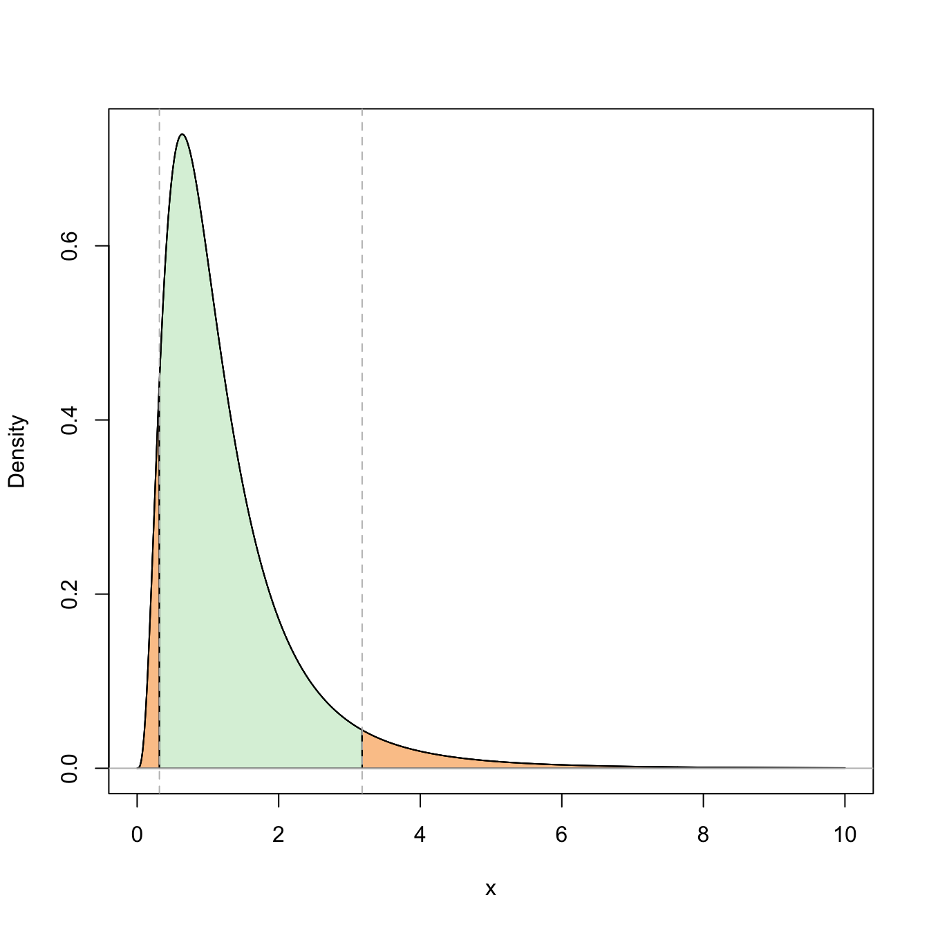
$Representation of the probability $\mathbb{P}(\mathcal{F}_{n_1-1,n_2-1;1-\alpha/2}\leq \mathcal{F}_{n_1-1,n_2-1}\leq \mathcal{F}_{n_1-1,n_2-1;\alpha/2})=1-\alpha$ (in green) and its complementary (in orange) for $\alpha=0.10$ and $n_1=n_2=10$.$

Figure 5.6: Representation of the probability $\mathbb{P}(\mathcal{F}_{n_1-1,n_2-1;1-\alpha/2}\leq \mathcal{F}_{n_1-1,n_2-1}\leq \mathcal{F}_{n_1-1,n_2-1;\alpha/2})=1-\alpha$ (in green) and its complementary (in orange) for $\alpha=0.10$ and $n_1=n_2=10$.

Then, a confidence interval for $\theta=\sigma_1^2/\sigma_2^2$ is

\[\begin{align*} \mathrm{CI}_{1-\alpha}(\sigma_1^2/\sigma_2^2)=\left[\frac{S_1'^2/S_2'^2}{\mathcal{F}_{n_1-1,n_2-1;\alpha/2}}, \frac{S_1'^2/S_2'^2}{\mathcal{F}_{n_1-1,n_2-1;1-\alpha/2}}\right]. \end{align*}\]

Remark. When using the tabulated probabilities for the Snedecor’s $\mathcal{F}$ distribution, usually the critical values of the distribution are only available for small probabilities $\alpha.$ However, a useful fact is that if $F\sim \mathcal{F}_{\nu_1,\nu_2},$ then $F'=1/F\sim\mathcal{F}_{\nu_2,\nu_1}.$ Therefore, if $\mathcal{F}_{\nu_1,\nu_2;\alpha}$ is the critical value $\alpha$ of $\mathcal{F}_{\nu_1,\nu_2},$ then

\[\begin{align*} \mathbb{P}(\mathcal{F}_{\nu_1,\nu_2}>\mathcal{F}_{\nu_1,\nu_2;\alpha})=\alpha &\iff \mathbb{P}(\mathcal{F}_{\nu_2,\nu_1}<1/\mathcal{F}_{\nu_1,\nu_2;\alpha})=\alpha\\ &\iff \mathbb{P}(\mathcal{F}_{\nu_2,\nu_1}>1/\mathcal{F}_{\nu_1,\nu_2;\alpha})=1-\alpha. \end{align*}\]

This means that

\[\begin{align*} \mathcal{F}_{\nu_2,\nu_1;1-\alpha}=1/\mathcal{F}_{\nu_1,\nu_2;\alpha}. \end{align*}\]

Obtaining the critical values for the $\mathcal{F}$ distribution can be easily done with the function qf(), as illustrated in Example 2.12.

Example 5.7 Two learning methods are applied for teaching children in the school how to read. The results of both methods were compared in a reading test at the end of the learning period. The resulting means and quasivariances of the tests are collected in the table below. Assuming that the results have a normal distribution, we want to obtain a confidence interval with confidence level $0.95$ for the mean difference.

Statistic	Method 1	Method 2
$n_i$	$11$	$14$
$\bar{X}_i$	$64$	$69$
$S_i'^2$	$52$	$71$

In the first place we have to verify if the two unknown variances are equal to see if we can apply the confidence intervals seen in Section 5.3.2. For that, we compute the confidence interval for the ratio of variances, and if that confidence interval contains the one, then this would indicate that there is no evidence against the assumption of equal variances. If that was the case, we can construct the confidence interval given in Section 5.3.2.⁶⁹

The sample quasivariances are

\[\begin{align*} S_1'^2=52,\quad S_2'^2=71. \end{align*}\]

Then, since $\mathcal{F}_{10,13;0.975}=1/\mathcal{F}_{13,10;0.025},$ the confidence interval at $0.95$ for the ratio of variances is

\[\begin{align*} \left[\frac{52/71}{\mathcal{F}_{10,13;0.025}},\frac{52/71}{\mathcal{F}_{10,13;0.975}}\right] \approx\left[\frac{0.73}{3.25},\frac{0.73}{1/3.58}\right]\approx[0.22,2.61]. \end{align*}\]

In R, the confidence interval for the ratio of variances can be computed as:

# n1, n2, S1'^2, S2'^2, alpha, c1, c2
n_1 <- 11
n_2 <- 14
S2_prime_1 <- 52
S2_prime_2 <- 71
alpha <- 0.05
c1 <- qf(1 - alpha / 2, df1 = n_1 - 1, df2 = n_2 - 1, lower.tail = FALSE)
c2 <- qf(alpha / 2, df1 = n_1 - 1, df2 = n_2 - 1, lower.tail = FALSE)

# CI
(S2_prime_1 / S2_prime_2) / c(c2, c1)
## [1] 0.2253751 2.6243088

The value one is inside the confidence interval, so the confidence interval does not provide any evidence against the hypothesis of the equality of variances. Therefore, we can use the confidence interval for unknown and equal variances.

The estimated variance is

\[\begin{align*} S^2=\frac{10\times 52+13\times 71}{11+14-2}\approx62.74. \end{align*}\]

Since the critical value is $t_{23;0.025}\approx2.069,$ the interval is

\[\begin{align*} \mathrm{CI}_{0.95}(\mu_1-\mu_2)=\left[(64-69)\mp t_{23;0.025} S\sqrt{\frac{1}{11}+\frac{1}{14}}\right]\approx[-11.6, 1.6]. \end{align*}\]

In R:

# Xbar1, Xbar2, S^2, t_{alpha/2;n1-n2-2}
X_bar_1 <- 64
X_bar_2 <- 69
S2 <- ((n_1 - 1) * S2_prime_1 + (n_2 - 1) * S2_prime_2) / (n_1 + n_2 - 2)
t <- qt(1 - alpha / 2, df = n_1 + n_2 - 2, lower.tail = TRUE)

# CI
(X_bar_1 - X_bar_2) + c(-1, 1) * t * sqrt(S2 * (1 / n_1 + 1 / n_2))
## [1] -11.601878   1.601878

This is a particular case of Proposition 1.11.↩︎
This reasoning is not fully rigorous. Using confidence intervals in a chained way may result in a confidence level that is not the nominal one. A more rigorous approach is possible with a confidence interval for $\mu_1-\mu_2$ with $\sigma_1^2\neq\sigma_2^2$ unknown, but it is beyond the scope of this course.↩︎

Statistic	Method 1	Method 2
\(n_i\)	\(11\)	\(14\)
\(\bar{X}_i\)	\(64\)	\(69\)
\(S_i'^2\)	\(52\)	\(71\)

Procedure	Measurements
Standard	\(32 \qquad 37 \qquad 35 \qquad 28 \qquad 41 \qquad 44 \qquad 35 \qquad 31 \qquad 34\)
New	\(35 \qquad 31 \qquad 29 \qquad 25 \qquad 34 \qquad 40 \qquad 27 \qquad 32 \qquad 31\)