2.1 Basic definitions
As seen in Example 1.3, employing frequentist ideas we can state that there is an underlying probability law that drives any random experiment. The interest of statistical inference when studying a random phenomenon lies on learning this underlying distribution.
Usually, for certain kinds of experiments and random variables, experience provides some information about the underlying distribution \(F\) (identified here with the cdf). In many situations, \(F\) is not exactly known, but we may know the approximate form of \(F\) up to a parameter \(\theta\) that drives its shape. In other words, we may know that \(F\) belongs to a parametric family of distributions \(\{F(\cdot;\theta): \theta\in\Theta\}\) that is indexed by a certain parameter \(\theta\in\Theta.\) For example, the class of distributions is \(\{\Phi(\cdot/\sigma):\sigma\in\mathbb{R}_+\}\) (remember Example 1.17) contains all the normal distributions \(\mathcal{N}(0,\sigma^2)\) and is indexed by the standard deviation parameter \(\sigma.\)
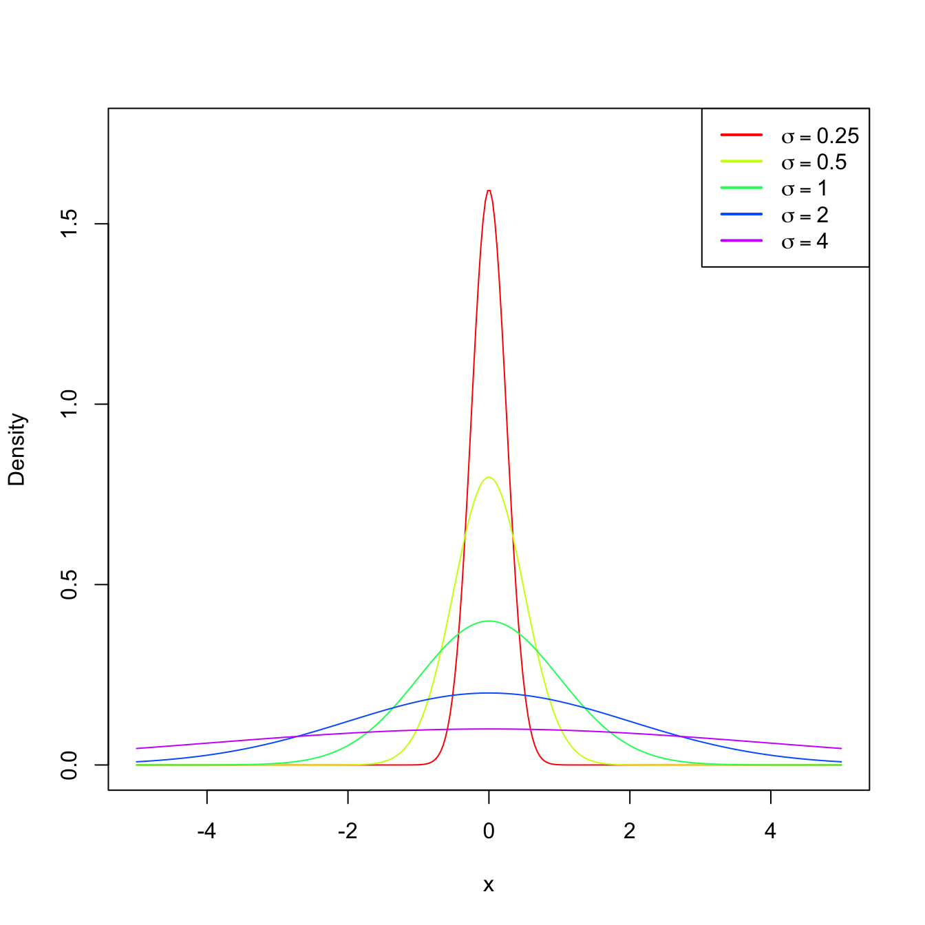
Figure 2.2: \(\mathcal{N}(0,\sigma^2)\) pdf’s for several standard deviations \(\sigma.\)
If our objective is to know more about \(F\) or, equivalently, about its driving parameter \(\theta,\) we can perform independent realizations of the experiment and then process the information in a certain way to infer knowledge about \(F\) or \(\theta.\) This is the process of performing statistical inference about \(F\) or, equivalently, about \(\theta.\) The fact that we perform independent repetitions of the experiment means that, for each repetition of the experiment, we have an associated rv with the same distribution \(F.\) This is the concept of a simple random sample.
Definition 2.1 (Simple random sample and sample realization) A simple random sample (srs) of size \(n\) of a rv \(X\) with distribution \(F\) is a collection of rv’s \((X_1,\ldots,X_n)\) that are independent and identically distributed (iid) with the distribution \(F.\) A sample realization are the observed values \((x_1,\ldots,x_n)\) of \((X_1,\ldots,X_n).\)
Therefore, a srs is a random vector \(\boldsymbol{X}=(X_1,X_2,\ldots,X_n)'\) that is defined over the measurable product space \((\mathbb{R}^n,\mathcal{B}^n).\) Since the rv’s are independent, the cdf of the sample (or of the random vector \(\boldsymbol{X}\)) is
\[\begin{align*} F_{\boldsymbol{X}}(x_1,x_2,\ldots,x_n)=F(x_1)F(x_2)\cdots F(x_n). \end{align*}\]
Example 2.1 We analyze next the underlying probability functions that appear in Example 1.3.
Consider the family of pmf’s given by \[\begin{align*} \mathbb{P}(X=1)=\theta, \quad \mathbb{P}(X=0)=1-\theta,\quad \theta\in [0,1]. \end{align*}\] The pmf of the first experiment in Example 1.3 belongs to this family, for \(\theta=0.5.\)
From previous experience, it is known that the rv that measures the number of events happening in a given time interval has a pmf that belongs to \(\{p(\cdot;\lambda):\lambda\in\mathbb{R}_+\},\) where
\[\begin{align} p(x;\lambda)=\frac{\lambda^x e^{-\lambda}}{x!}, \quad x=0,1,2,3,\ldots\tag{2.1} \end{align}\] This is the pmf of the Poisson of intensity parameter \(\lambda\) that was introduced in Exercise 1.14. Replacing \(\lambda=4\) and \(x=0,1,2,3,\ldots\) in (2.1), we obtain the following probabilities:
\(x\) \(0\) \(1\) \(2\) \(3\) \(4\) \(5\) \(6\) \(7\) \(8\) \(\geq 9\) \(p(x;4)\) \(0.018\) \(0.073\) \(0.147\) \(0.195\) \(0.156\) \(0.156\) \(0.104\) \(0.060\) \(0.030\) \(0.021\) Observe that these probabilities are similar to the relative frequencies given in Table 1.2.
From previous experience, it is known that the rv that measures the weight of a person follows a normal distribution \(\mathcal{N}(\mu,\sigma^2),\) whose pdf is \[\begin{align*} \phi(x;\mu,\sigma^2)=\frac{1}{\sqrt{2\pi\sigma^2}}\exp\left\{-\frac{(x-\mu)^2}{2\sigma^2}\right\},\quad \mu\in\mathbb{R}, \ \sigma^2\in\mathbb{R}_+. \end{align*}\] Indeed, setting \(\mu=39\) and \(\sigma=5,\) the next probabilities for the intervals are obtained:
\(I\) \((-\infty,35]\) \((35,45]\) \((45,55]\) \((55,65]\) \((65,\infty)\) \(\mathbb{P}(x\in I)\) \(0.003\) \(0.209\) \(0.673\) \(0.114\) \(0.001\) Observe the similarity with Table 1.3.
Given a srs \(X_1,\ldots,X_n,\) inference is carried out by means of “summaries” of this sample. The general definition of such summary is called statistic, and is another key pillar in statistical inference.
Definition 2.2 (Statistic) A statistic \(T\) is any measurable function \(T:(\mathbb{R}^n,\mathcal{B}^n)\rightarrow(\mathbb{R}^k,\mathcal{B}^k),\) where \(k\) is the dimension of the statistic.
A vastness of statistics is possible given a srs. Definitely not all of them will be as useful for inferential purposes! In particular, the sample itself is always a statistic, but surely not the most interesting one as it does not summarize information about a parameter \(\theta.\)
Example 2.2 The following are examples of statistics:
- \(T_1(X_1,\ldots,X_n)=\frac{1}{n}\sum_{i=1}^n X_i.\)
- \(T_2(X_1,\ldots,X_n)=\frac{1}{n}\sum_{i=1}^n (X_i-\bar{X})^2.\)
- \(T_3(X_1,\ldots,X_n)=\min\{X_1,\ldots,X_n\}=: X_{(1)}.\)
- \(T_4(X_1,\ldots,X_n)=\max\{X_1,\ldots,X_n\}=: X_{(n)}.\)
- \(T_5(X_1,\ldots,X_n)=\sum_{i=1}^n \log X_i.\)
- \(T_6(X_1,\ldots,X_n)=(X_{(1)},X_{(n)})'.\)
- \(T_7(X_1,\ldots,X_n)=(X_1,\ldots,X_n)'.\)
All the statistics have dimension \(k=1,\) except \(T_6\) with \(k=2\) and \(T_7\) with \(k=n.\)
From the definition, we can see that a statistic is a rv, or a random vector if \(k>1.\) This new rv is a transformation (see Section 1.4) of the random vector \((X_1,\ldots,X_n)'.\) The distribution of the statistic \(T\) is called the sampling distribution of \(T\), since it depends on the distribution of the sample and the transformation considered.
We see next some examples on the determination of the sampling distribution of statistics for discrete and continuous rv’s.
Example 2.3 A coin is tossed independently three times. Let \(X_i,\) \(i=1,2,3,\) be the rv that measures the outcome of the \(i\)-th toss:
\[\begin{align*} X_i=\begin{cases} 1 & \text{if H is the outcome of the $i$-th toss},\\ 0 & \text{if T is the outcome of the $i$-th toss}. \end{cases} \end{align*}\]
If we do not know whether the coin is fair (Heads and Tails may not be equally likely), then the pmf of \(X_i\) is given by
\[\begin{align*} \mathbb{P}(X_i=1)=\theta,\quad \mathbb{P}(X_i=0)=1-\theta, \quad \theta\in\Theta=[0,1]. \end{align*}\]
The three rv’s are independent. Therefore, the probability of the sample \((X_1,X_2,X_3)\) is the product of the individual probabilities of \(X_i,\) that is,
\[\begin{align*} \mathbb{P}(X_1=x_1,X_2=x_2,X_3=x_3)=\mathbb{P}(X_1=x_1)\mathbb{P}(X_2=x_2)\mathbb{P}(X_3=x_3). \end{align*}\]
The following table collects the values of the pmf of the sample for each possible value of the sample.
| \((x_1,x_2,x_3)\) | \(p(x_1,x_2,x_3)\) |
|---|---|
| \((1,1,1)\) | \(\theta^3\) |
| \((1,1,0)\) | \(\theta^2(1-\theta)\) |
| \((1,0,1)\) | \(\theta^2(1-\theta)\) |
| \((0,1,1)\) | \(\theta^2(1-\theta)\) |
| \((1,0,0)\) | \(\theta(1-\theta)^2\) |
| \((0,1,0)\) | \(\theta(1-\theta)^2\) |
| \((0,0,1)\) | \(\theta(1-\theta)^2\) |
| \((0,0,0)\) | \((1-\theta)^3\) |
We can define the sum statistic as \(T_1(X_1,X_2,X_3)=\sum_{i=1}^3 X_i.\) Now, from the previous table, we can compute the sampling distribution of \(T\) as the pmf given by
| \(t_1=T_1(x_1,x_2,x_3)\) | \(p(t_1)\) |
|---|---|
| \(3\) | \(\theta^3\) |
| \(2\) | \(3\theta^2(1-\theta)\) |
| \(1\) | \(3\theta(1-\theta)^2\) |
| \(0\) | \((1-\theta)^3\) |
To compute the table, we have summed the probabilities \(p(x_1,x_2,x_3)\) of the cases \((x_1,x_2,x_3)\) leading to each value of \(t_1.\)
Another possible statistic is the sample mean, \(T_2(X_1,X_2,X_3)=\bar{X},\) whose sampling distribution is
| \(t_2=T_2(x_1,x_2,x_3)\) | \(p(t_2)\) |
|---|---|
| \(1\) | \(\theta^3\) |
| \(2/3\) | \(3\theta^2(1-\theta)\) |
| \(1/3\) | \(3\theta(1-\theta)^2\) |
| \(0\) | \((1-\theta)^3\) |
Example 2.4 Let \((X_1,\ldots,X_n)\) be a srs of a rv with \(\mathrm{Exp}(\theta)\) distribution, that is, with pdf
\[\begin{align*} f(x;\theta)= \theta e^{-\theta x}, \quad x>0, \ \theta>0. \end{align*}\]
We will obtain the sampling distribution of the sum statistic \(T(X_1,\ldots,X_n)=\sum_{i=1}^n X_i.\)
First, observe that \(\mathrm{Exp}(\theta)\stackrel{d}{=}\Gamma(1,1/\theta)\) since the pdf of a \(\Gamma(\alpha,\beta)\) is given by
\[\begin{align} f(x;\alpha,\beta)=\frac{1}{\Gamma(\alpha) \beta^{\alpha}}\, x^{\alpha-1} e^{-x/\beta}, \quad x>0, \ \alpha>0, \ \beta>0. \tag{2.2} \end{align}\]
From Exercise 1.21 we know that the sum of \(n\) independent rv’s \(\Gamma(\alpha,\beta)\) is a \(\Gamma(n\alpha,\beta)\) without the need of using transformations. Therefore, thanks to this shortcut, the distribution of the sum statistic \(T(X_1,\ldots,X_n)=\sum_{i=1}^n X_i\) is a \(\Gamma(n,1/\theta).\)
Example 2.5 Let \((X_1,X_2)\) be a srs of a rv with uniform distribution \(\mathcal{U}(\theta-1,\theta+1),\) \(\theta>0.\) The pdf of this distribution is
\[\begin{align*} f(x;\theta)=\frac{1}{2} 1_{\{x\in(\theta-1,\theta+1)\}}. \end{align*}\]
We obtain the sampling distribution of the average statistic \(T(X_1,X_2)=(X_1+X_2)/2.\) To do so, we use Corollary 1.2 to have first the distribution of \(S=X_1+X_2\):
\[\begin{align*} f_S(s;\theta)&=\int_{\mathbb{R}} f(s-x;\theta)f(x;\theta)\,\mathrm{d} x\\ &=\frac{1}{4}\int_{\mathbb{R}} 1_{\{(s-x)\in(\theta-1,\theta+1)\}}1_{\{x\in(\theta-1,\theta+1)\}}\,\mathrm{d} x\\ &=\frac{1}{4}\int_{\mathbb{R}} 1_{\{x\in(s-\theta-1,s-\theta+1)\}}1_{\{x\in(\theta-1,\theta+1)\}}\,\mathrm{d} x\\ &=\frac{1}{4}\int_{\mathbb{R}} 1_{\{x\in(\max(s-\theta-1,\theta-1),\min(s-\theta+1,\theta+1)\}}\,\mathrm{d} x\\ &=\frac{\min(s-\theta+1,\theta+1)-\max(s-\theta-1,\theta-1)}{4} \end{align*}\]
with \(s\in(2(\theta-1),2(\theta+1)).\) Using Exercise 1.33, the pdf of \(T=S/2\) is therefore
\[\begin{align} f_T(t;\theta)=\frac{\min(2t-\theta+1,\theta+1)-\max(2t-\theta-1,\theta-1)}{2} \tag{2.3} \end{align}\]
with \(t\in(\theta-1,\theta+1).\)
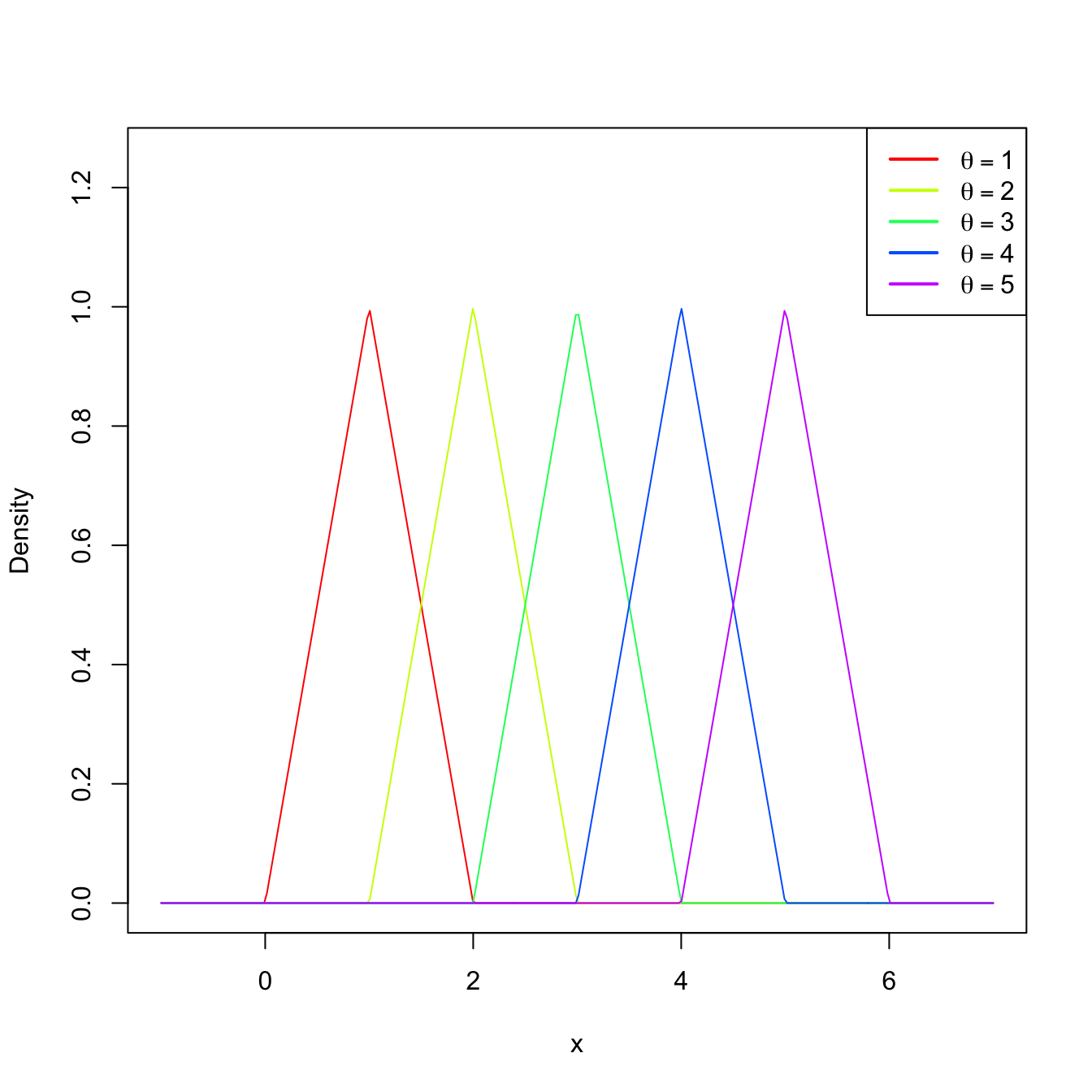
Figure 2.3: Pdf (2.3) for several values of \(\theta.\)
Example 2.6 (Sampling distribution of the minimum) Let \((X_1,\ldots,X_n)\) be a srs of a rv with cdf \(F\) (either discrete or continuous). The sampling distribution of the statistic \(T(X_1,\ldots,X_n)=X_{(1)}\) follows from the cdf of \(T\) using the iid-ness of the sample and the properties of the minimum:
\[\begin{align*} 1-F_T(t) &=\mathbb{P}_T(T>t)=\mathbb{P}_{(X_1,\ldots,X_n)}(X_{(1)}> t)\\ &=\mathbb{P}_{(X_1,\ldots,X_n)}(X_1> t,\ldots,X_n> t)=\prod_{i=1}^n \mathbb{P}_{X_i}(X_i> t)\\ &=\prod_{i=1}^n\left[1-F_{X_i}(t)\right]=\left[1-F(t)\right]^n. \end{align*}\]