4.1 Method of moments

Consider a population $X$ whose distribution depends on $K$ unknown parameters $\boldsymbol{\theta}=(\theta_1,\ldots,\theta_K)'.$ If they exist, the population moments are, in general, functions of the unknown parameters $\boldsymbol{\theta}.$ That is,

\[\begin{align*} \alpha_r\equiv\alpha_r(\theta_1,\ldots,\theta_K):=\mathbb{E}[X^r], \quad r=1,2,\ldots \end{align*}\]

Given a srs of $X,$ we denote by $a_r$ to the sample moment of order $r$ that estimates $\alpha_r$:

\[\begin{align*} a_r:=\bar{X^r}=\frac{1}{n}\sum_{i=1}^n X_i^r, \quad r=1,2,\ldots \end{align*}\]

Note that the sample moments do not depend on $\boldsymbol{\theta}=(\theta_1,\ldots,\theta_K)'$ but the population moments do. This is the key fact that the method of moments exploits for finding the values of the parameters $\boldsymbol{\theta}$ that perfectly equate $\alpha_r$ to $a_r$ for as many $r$’s as necessary.⁴² The overall idea can be abstracted as matching population with sample moments and solving for $\boldsymbol{\theta}$.

Definition 4.1 (Method of moments) Let $X\sim F_{\boldsymbol{\theta}}$ with $\boldsymbol{\theta}=(\theta_1,\ldots,\theta_K)'.$ From a srs of $X,$ the method of moments produces the estimator $\hat{\boldsymbol{\theta}}_{\mathrm{MM}}$ that is the solution to the system of equations

\[\begin{align*} \alpha_r(\theta_1,\ldots,\theta_K)=a_r, \quad r=1,\ldots, R, \end{align*}\]

where $R\geq K$ is the lowest integer such that the system admits a unique solution and $\theta_1,\ldots,\theta_K$ are the variables. The estimator $\hat{\boldsymbol{\theta}}_{\mathrm{MM}}$ is simply referred to as the moment estimator of $\boldsymbol{\theta}.$

Example 4.1 Assume that we have a population with distribution $\mathcal{N}(\mu,\sigma^2)$ and a srs $(X_1,\ldots,X_n)$ from it. In this case, $\boldsymbol{\theta}=(\mu,\sigma^2)'.$ Let us compute the moment estimators of $\mu$ and $\sigma^2.$

For estimating two parameters, we need at least a system with two equations. We compute in the first place the first two moments of the rv $X\sim \mathcal{N}(\mu,\sigma^2).$ The first one is $\alpha_1(\mu,\sigma^2)=\mathbb{E}[X]=\mu.$ The second order moment arises from the variance $\sigma^2$:

\[\begin{align*} \alpha_2(\mu,\sigma^2)=\mathbb{E}[X^2]=\mathbb{V}\mathrm{ar}[X]+\mathbb{E}[X]^2=\sigma^2+\mu^2. \end{align*}\]

On the other hand, the first two sample moments are given by

\[\begin{align*} a_1=\bar{X}, \quad a_2=\frac{1}{n}\sum_{i=1}^n X_i^2=\bar{X^2}. \end{align*}\]

Then, the equations to solve in $(\mu,\sigma^2)$ are

\[\begin{align*} \begin{cases} \mu=\bar{X},\\ \sigma^2+\mu^2=\bar{X^2}. \end{cases} \end{align*}\]

The solution for $\mu$ is already in the first equation. Substituting this value in the second equation and solving $\sigma^2,$ we get the estimators

\[\begin{align*} \hat{\mu}_{\mathrm{MM}}=\bar{X},\quad \hat{\sigma}^2_{\mathrm{MM}}=\bar{X^2}-\hat{\mu}_{\mathrm{MM}}^2=\bar{X^2}-\bar{X}^2=S^2. \end{align*}\]

It turns out the sample mean and sample variance are the moment estimators of $(\mu,\sigma^2).$

Example 4.2 Let $(X_1,\ldots,X_n)$ be a srs of a rv $X\sim\mathcal{U}(0,\theta).$ Let us obtain the estimator of $\theta$ by the method of moments.

The first population moment is $\alpha_1(\theta)=\mathbb{E}[X]=\theta/2$ and the first sample moment is $a_1=\bar{X}.$ Equating both and solving for $\theta,$ we readily obtain $\hat{\theta}_{\mathrm{MM}}=2\bar{X}.$

We can observe that the estimator $\hat{\theta}_{\mathrm{MM}}$ of the upper range limit can be actually smaller than $X_{(n)}.$ Or larger than $\theta,$⁴³ even if we do not have any possible information on the sample above $\theta.$ than the maximum observation. Then, intuitively, the estimator is clearly suboptimal. This observation is just an illustration of a more general fact that shows that the estimators obtained by the method of moments are usually not the most efficient ones.

Example 4.3 Let $(X_1,\ldots,X_n)$ be a srs of a rv $X\sim\mathcal{U}(-\theta,\theta),$ $\theta>0.$ Obtain the moment estimator of $\theta.$

The first population moment is now $\alpha_1(\theta)=\mathbb{E}[X]=0.$ It does not contain any information about $\theta$! Therefore, we need to look into the second population moment, that is $\alpha_2(\theta)=\mathbb{E}[X^2]=\mathbb{V}\mathrm{ar}[X]+\mathbb{E}[X]^2=\mathbb{V}\mathrm{ar}[X]=\theta^2/3.$ With this moment we can now solve $\alpha_2(\theta)=\bar{X^2}$ for $\theta,$ obtaining $\hat{\theta}_{\mathrm{MM}}=\sqrt{3\bar{X^2}}.$

This example illustrates that in certain situations it may be required to consider $R>K$ equations (here, $R=2$ and $K=1$) to compute the moment estimators if some of them are non-informative.

Example 4.4 We know from (2.7) that $\mathbb{E}[\chi^2_\nu]=\nu.$ Therefore, it is immediate that $\hat{\nu}_{\mathrm{MM}}=\bar{X}.$ Figure 4.2 shows a visualization of how the method of moments operates in this case: it “scans” several degrees of freedom $\nu$ until finding that for which $\nu=\bar{X}.$ In this process, the method of moments only uses the information of the sample realization $x_1,\ldots,x_n$ that is summarized in $\bar{X},$ nothing else.⁴⁴

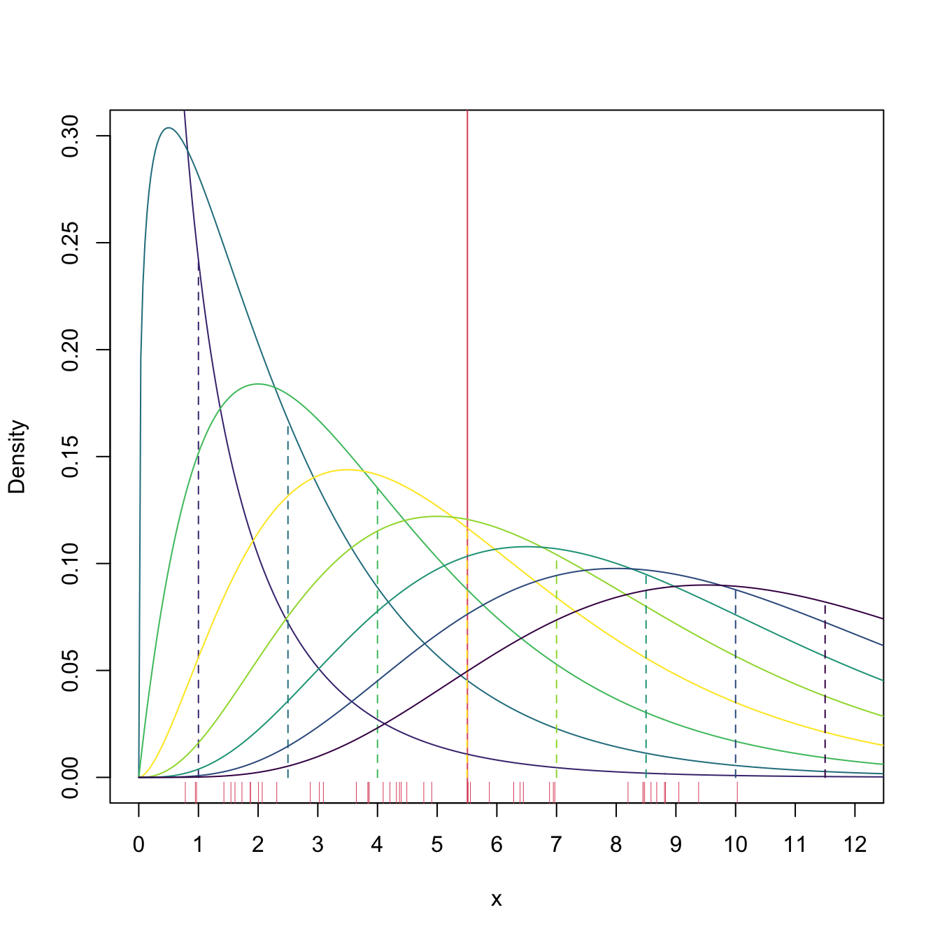
$$\chi^2_\nu$ densities for several degrees of freedom $\nu.$ Their color varies according to how far away the expectation $\nu$ (shown in the vertical dashed lines) is from $\bar{X}\approx5.5$ (red vertical line): the more yellowish, the closer $\nu$ is to $\bar{X}$.$

Figure 4.2: $\chi^2_\nu$ densities for several degrees of freedom $\nu.$ Their color varies according to how far away the expectation $\nu$ (shown in the vertical dashed lines) is from $\bar{X}\approx5.5$ (red vertical line): the more yellowish, the closer $\nu$ is to $\bar{X}$.

An important observation is that, if the parameters to be estimated $\theta_1,\ldots,\theta_K$ can be written as a function of $K$ population moments through continuous functions,

\[\begin{align*} \theta_k=g_k(\alpha_1,\ldots,\alpha_K), \quad k=1,\ldots,K, \end{align*}\]

then the estimator of $\theta_k$ by the method of moments simply follows by replacing $\alpha$’s by $a$’s:

\[\begin{align*} \hat{\theta}_{\mathrm{MM},k}=g_k(a_1,\ldots,a_K). \end{align*}\]

Recall that $g_k$ is such that $\theta_k=g_k\left(\alpha_1(\theta_1,\ldots,\theta_K),\ldots,\alpha_K(\theta_1,\ldots,\theta_K)\right).$ That is, $g_k$ is the $k$-th component of the inverse function of

\[\begin{align*} \alpha:(\theta_1,\ldots,\theta_K)\in\mathbb{R}^K\mapsto \left(\alpha_1(\theta_1,\ldots,\theta_K),\ldots,\alpha_K(\theta_1,\ldots,\theta_K)\right)\in\mathbb{R}^K. \end{align*}\]

Proposition 4.1 (Consistency in probability of the method of moments) Let $(X_1,\ldots,X_n)$ be a srs of a rv $X\sim F_{\boldsymbol{\theta}}$ with $\boldsymbol{\theta}=(\theta_1,\ldots,\theta_K)'$ that verifies

\[\begin{align} \mathbb{E}[(X^k-\alpha_k)^2]<\infty, \quad k=1,\ldots,K.\tag{4.1} \end{align}\]

If $\theta_k=g_k(\alpha_1,\ldots,\alpha_K),$ with $g_k$ continuous, then the moment estimator for $\theta_k,$ $\hat{\theta}_{\mathrm{MM},k}=g_k(a_1,\ldots,a_K),$ is consistent in probability:

\[\begin{align*} \hat{\theta}_{\mathrm{MM},k}\stackrel{\mathbb{P}}{\longrightarrow} \theta_k,\quad k=1,\ldots,K. \end{align*}\]

Proof (Proof of Proposition 4.1). Thanks to the condition (4.1), the LLN implies that the sample moments $a_1,\ldots,a_K$ are consistent in probability for estimating the population moments. In addition, the functions $g_k$ are continuous for all $k=1,\ldots,K,$ hence by Theorem 3.3, $\hat{\theta}_k$ is consistent in probability for $\theta_k,$ $k=1,\ldots,K.$

The principle of equating $\alpha_r$ to $a_r$ rests upon the fact that $a_r\stackrel{\mathbb{P}}{\longrightarrow}\alpha_r$ when $n\to\infty$ (see Corollary 3.2).↩︎
Assume $\theta=1$ and $n=2$ with $(x_1,x_2)=(0.5,0.75).$ Then, $\hat{\theta}_{\mathrm{MM}}=1.25,$ but we never observed a quantity above $1.25$ in the sample.↩︎
In particular, it does not use the form of the pdf.↩︎